Resampling and Bootstrap

PSTAT 234 (Fall 2025)

Sang-Yun Oh

University of California, Santa Barbara

Understanding Data as Distributions

• Finite number of units: census or sample survey
• Infinite number of units: e.g., physical experiments, simulations
• All can be thought of as distributions
• Population distribution \(F\) vs. empirical distribution \(\hat{F}\)
• Sample statistic estimates a population parameter. e.g., \(\bar{x}\) estimates \(\mu\).
• We can show if \(\mu = E_{F}(X)\), then \[\mu_\hat{F} = E_{\hat{F}}(X) = \bar{x}\]

Data: Random Sample

• Let \(\mathcal{U} = \{U_1, U_2, \dots, U_N\}\) be all individuals in the population.

• \(N\) can be finite or infinite.

• Denote \(n\) integers between \(1\) and \(N\) with equal probability as: \[ j_1,\ j_2,\ \dots,\ j_n \]

• Then, random sampling is defined as: \[ u_1 = U_{j_1},\ u_2 = U_{j_2},\ \dots,\ u_n = U_{j_n} \]

• Assume random sampling is with replacement

Data: Measurements from a Random Sample

• Let \(x_i\) be the value of the variable of interest for unit \(u_i\).

• Population - census measurements¹:
  \[\mathcal{X} = (X_1, X_2, \dots, X_N)\]

• Observed data - measurements: \[{\bf x} = (x_1, x_2, \dots, x_n).\]

• Observed data can have repeated values.

• We often draw histograms of measurements from random samples.

1. Here, \(X_i\) are not random variables

Histogram as Probability Functions

X = norm(loc=3, scale=1)

num_data = 100 # number of observations
num_bins = 20  # number of bins

x_data = X.rvs(num_data) # simulate data
bin_edges = np.linspace(-2, 8, num=num_bins+1)
bin_width = 10/num_bins

# histogram with density and counts
fhat, _ = np.histogram(x_data, bins=bin_edges, density=True)
counts, _ = np.histogram(x_data, bins=bin_edges, density=False)

Histogram Density

Histogram Counts

Properties of Histograms

• counts is a scaled discrete distribution (pmf) \[\sum_{b=1}^B \texttt{counts}_b = n\quad \Rightarrow \quad \sum_{b=1}^B \hat{p}(x_b) = 1, \] where \(\hat{p}(x_b) = \texttt{counts}_b/n\)

• fhat is a piecewise constant continuous distribution (pdf) \[\int_{-\infty}^{\infty} \hat{f}(y)\, dy = 1\quad \Rightarrow \quad \sum_{b=1}^B \hat{f}(x_b)\cdot \Delta x_b = 1\]

  sum(fhat*bin_width) # density times bin widths (0.5) adds up to 1

  1.0

Histograms as Probability Functions

When density=True, \(\hat f(y)\) is a piecewise constant approximation of \(f(y)\). In other words, histogram function is a continuous approximation of the pdf.

Estimating Probability Distributions

normalize_fhat  = fhat/sum(fhat)          # heights1: just normalizing fhat (constant bin width)
fhat_delta      = fhat*np.diff(bin_edges) # heights2: approximating integral with constant height per bin
bin_probability = counts/num_data         # heights3: probability of being in bin

assert(all(np.isclose(normalize_fhat, fhat_delta)))  # heights1 is equal to heights2
assert(all(np.isclose(fhat_delta, bin_probability))) # heights2 is equal to heights3

midpoints = bin_edges[:-1] + np.diff(bin_edges)
# Seaborn does not natively support step plots or stem plots, but we can use lineplot and scatter for approximation

# fig, ax = plt.subplots(1, 2, figsize=(20, 5))

x_grid = np.linspace(-2, 8, num=1000)

# Continuous approximation: true pdf and histogram density
sns.lineplot(x=x_grid, y=X.pdf(x_grid), label='pdf: f(x)')
sns.lineplot(x=midpoints, y=fhat, label='approx pdf: fhat', drawstyle='steps-pre')
plt.show()

# Discrete approximation: true probabilities and bin probabilities
ax1 =sns.scatterplot(x=midpoints, y=X.pdf(midpoints)*np.diff(bin_edges), marker='o', label='pmf: f*delta')
ax2 = sns.scatterplot(x=midpoints, y=bin_probability, marker='o', label='approx pmf: phat')
ax1.vlines(midpoints, 0, X.pdf(midpoints)*np.diff(bin_edges), color='C0')
ax2.vlines(midpoints, 0, bin_probability, color='C1')
plt.show()

Continuous Approximation

Discrete Approximation

Histogram with \(n\) nonzero bins

Empirical Distribution Function

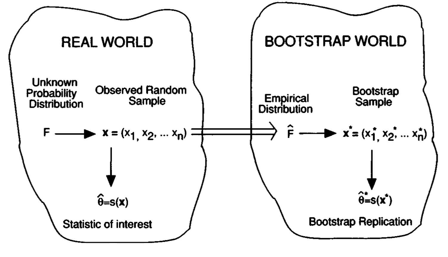
Having observed a random sample of size \(n\) from a probability distribution \(F\),

\[ F \rightarrow\left(x_1, x_2, \cdots, x_n\right) \]

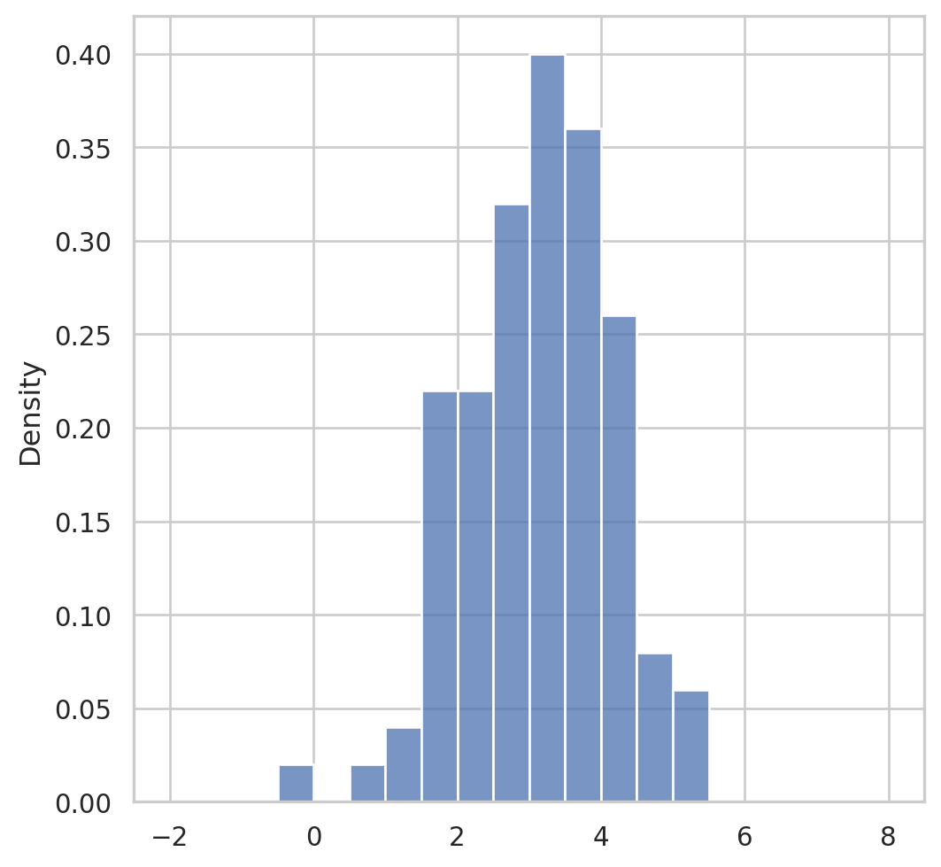
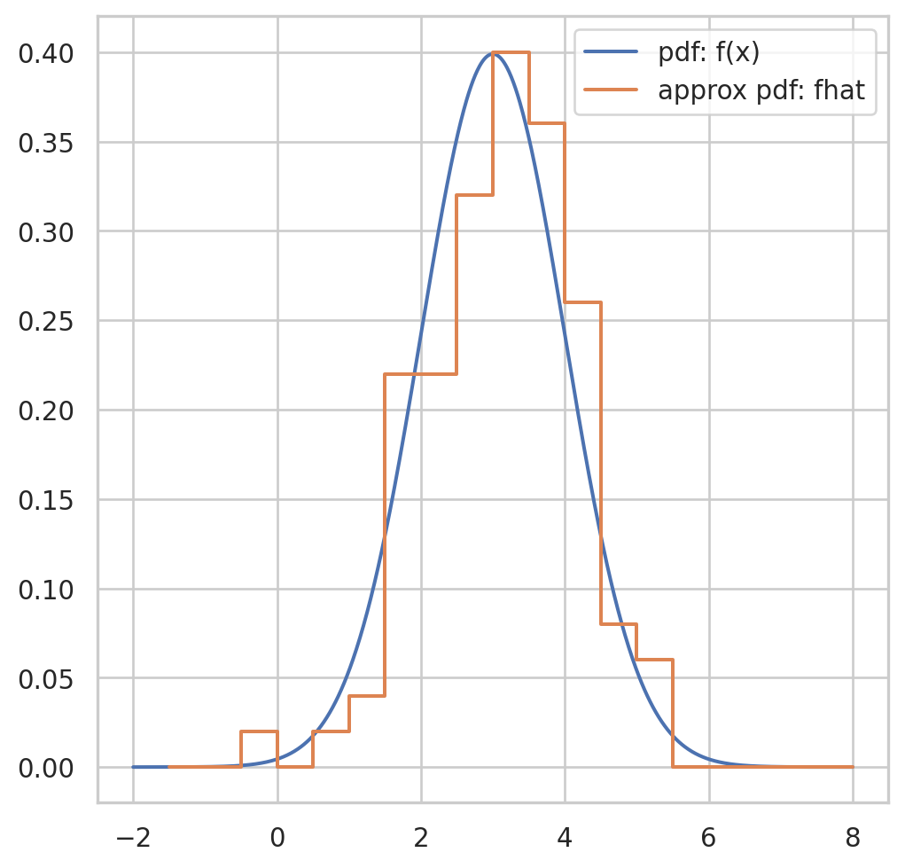
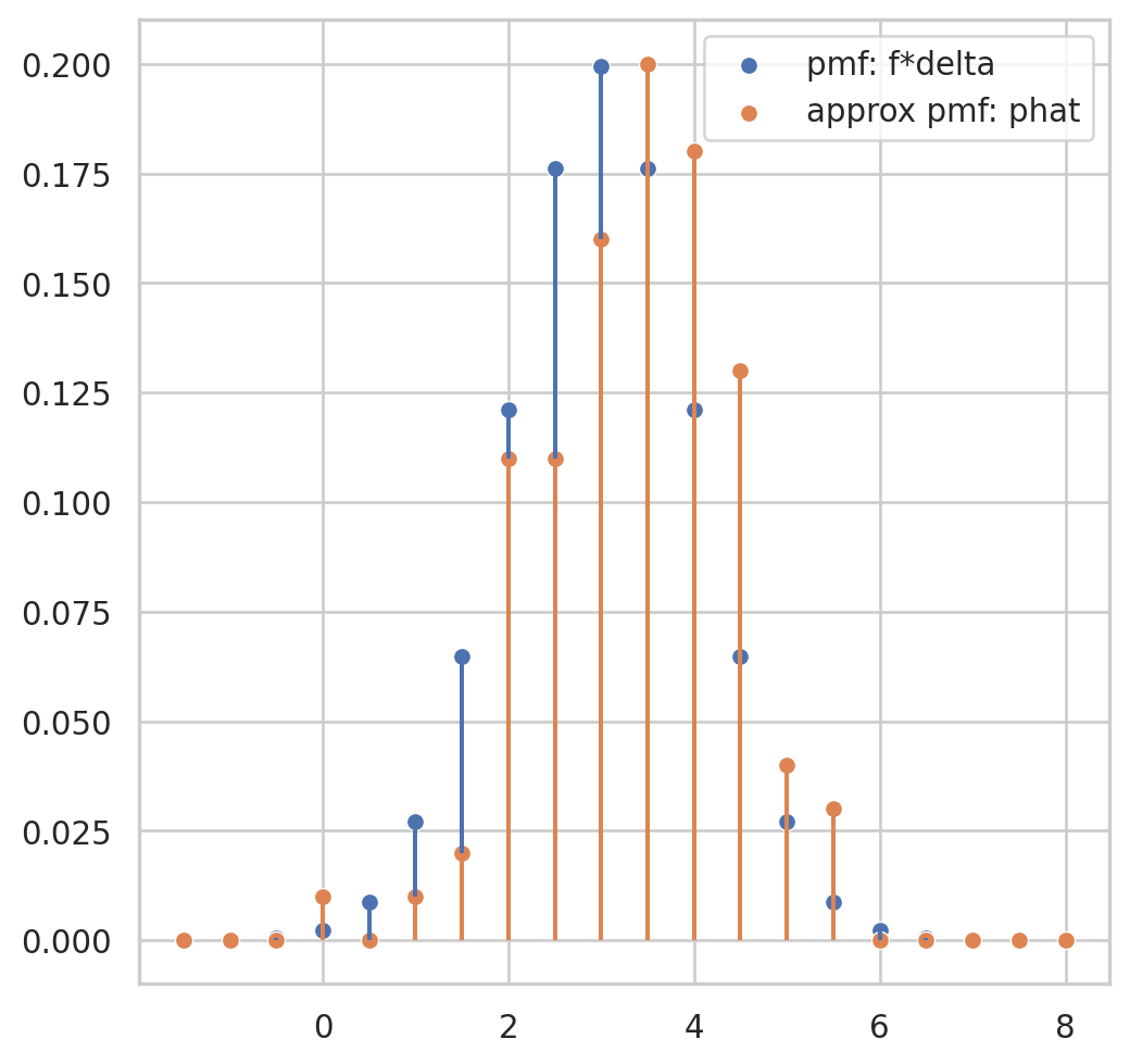
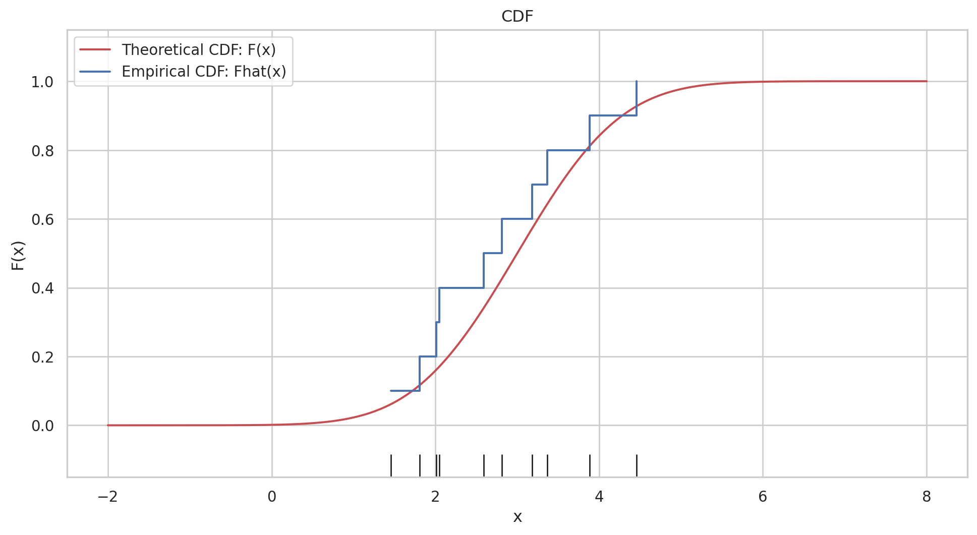
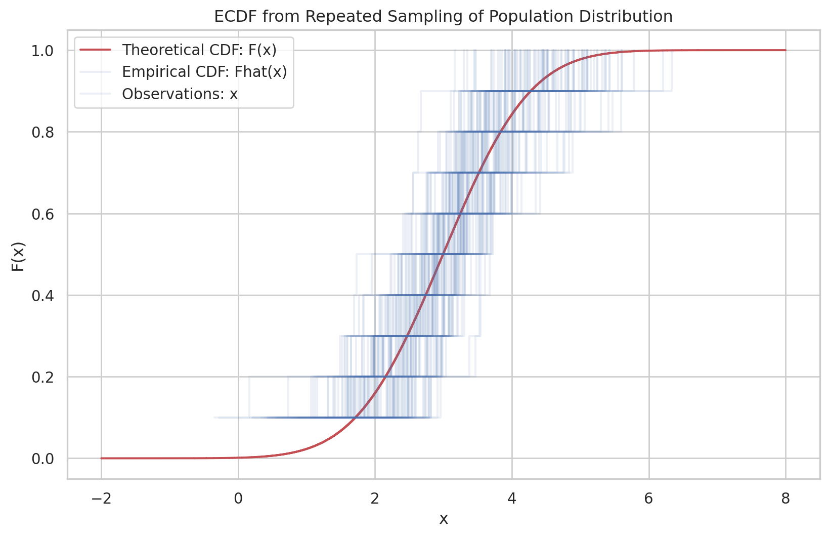
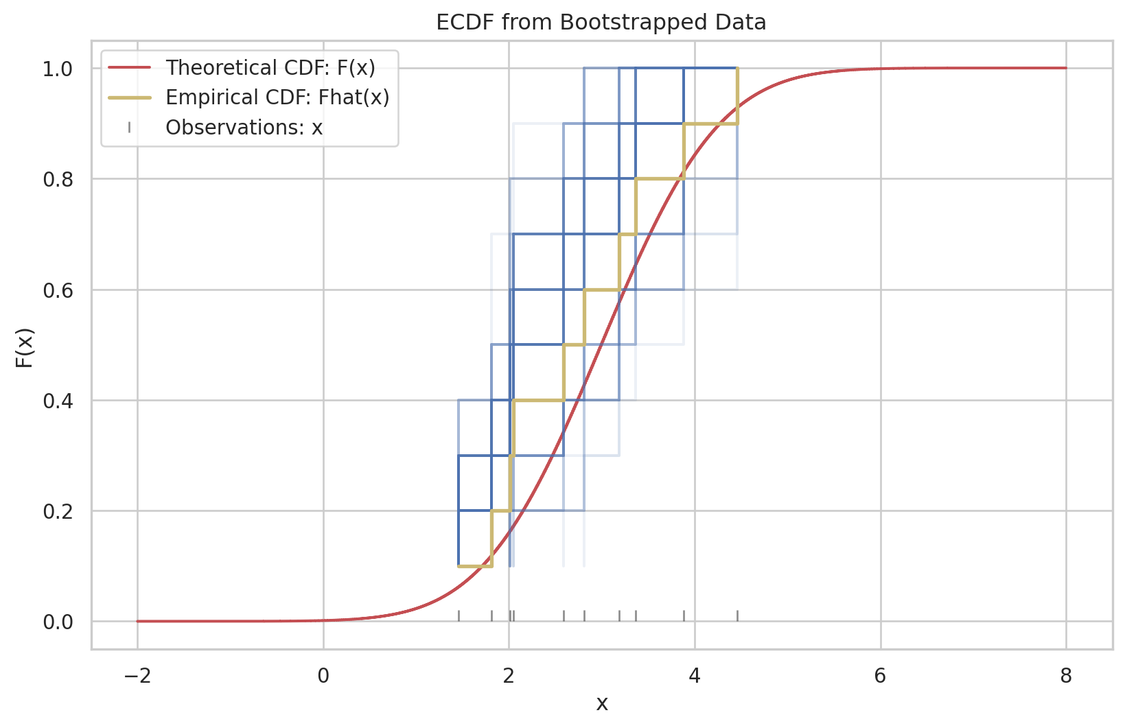
the empirical distribution function \(\hat{F}\) is defined to be the discrete distribution that puts probability \(1 / n\) on each value \(x_i, i=\) \(1,2, \cdots, n\). In other words, \(\hat{F}\) assigns to a set \(A\) in the sample space of \(x\) its empirical probability

\[ \widehat{\operatorname{Prob}}\{A\}=\#\left\{x_i \in A\right\} / n \]

the proportion of the observed sample \(\mathbf{x}=\left(x_1, x_2, \cdots, x_n\right)\) occurring in \(A\). We will also write \(\operatorname{Prob}_{\hat{F}}\{A\}\) to indicate \(\widehat{\operatorname{Prob}}\{A\}\). The hat symbol ” \(\wedge\) ” always indicates quantities calculated from the observed data.

Empirical distribution \(\hat{F}\) is a cumulative distribution function (CDF) with probability mass function (pmf) \(\hat{p}(x_i) = 1/n\) for \(i=1,2,\dots,n\).

Empirical CDF

def ecdf(data):
  x_ord = np.sort(data)
  n = x_ord.size
  Fhat = np.arange(1, n+1) / n
  
  return x_ord, Fhat

np.random.seed(233)

x_data = X.rvs(10) # simulate data
x_os, Fhat = ecdf(x_data)

fig, ax = plt.subplots(1, 1, figsize=(12, 6))

# Theoretical CDF as a lineplot
sns.lineplot(x=x_grid, y=X.cdf(x_grid), ax=ax, color='r', label='Theoretical CDF: F(x)')

# Empirical CDF as a step plot
ax.step(x_os, Fhat, where='post', color='b', label='Empirical CDF: Fhat(x)')

# Observations as rug plot
sns.rugplot(x=x_os, ax=ax, height=0.05, color='k')

ax.set_title('CDF')
ax.set_xlabel('x')
ax.set_ylabel('F(x)')
ax.legend()
plt.show()

Empirical Cumulative Distribution Function

• Recall our data \(x_i\), where \(i=1,2,\dots,n\) and order statistic, \(x_{(i)}\).

• Empirical CDF is defined as: \[ F(x) = P(X\leq x) = \int_{-\infty}^x f(z)\, dz \]

• We can approximate \(F(x)\) with \(\hat F(x)\) at discrete points \(x_{(i)}\) as: \[ \begin{aligned} &\hat P(X< x_{(1)}) = 0\\ \hat F(x_{(1)}) = &\hat P(X\leq x_{(1)}) = 1/n\\ \hat F(x_{(2)}) = &\hat P(X\leq x_{(2)}) = 2/n\\ &\vdots \\ \hat F(x_{(n)}) = &\hat P(X\leq x_{(n)}) = n/n = 1\\ \end{aligned} \]

Parameter vs. Statistic

• A parameter is a numerical characteristic of the population or true distribution, e.g., mean, variance, quantiles, etc.

• A statistic is a numerical characteristic of a sample, e.g., sample mean, sample variance, sample quantiles, etc.

• A statistic is used to estimate a parameter.

Example: Sample Mean

For a discrete approximation \(\hat{F}(x) = \hat p(x_i) = 1/n\), of a continuous distribution \(F\),

• \(\mu_F = E_F(X)\) is a parameter.
• \(\hat{\mu}_{\hat{F}} = E_{\hat{F}}(X)\) is called a plug-in estimator

\[\hat{\mu}_{\hat{F}} = \underbrace{E_{\hat{F}}(X) = \sum_{i=1}^n x_i \cdot \hat{p}(x_i)}_\text{Plugin Estimator} = \underbrace{\frac{1}{n} \sum_{i=1}^n x_i = \bar{x}}_\text{Sample Statistic}\]

Example: Sample Variance

• \(\sigma^2_F = \text{Var}_F(X) = E_F[(X - \mu_F)^2]\) is a parameter.
• \(\hat{\sigma}^2_{\hat{F}} = \text{Var}_{\hat{F}}(X) = E_{\hat{F}}[(X - \hat{\mu}_{\hat{F}})^2]\) is called a plug-in estimator

\[ \begin{aligned} \hat{\sigma}_{\hat{F}}^2 &= \overbrace{E_{\hat{F}}[(X - \hat{\mu}_{\hat{F}})^2] = \sum_{i=1}^n (x_i - \hat{\mu}_{\hat{F}})^2 \cdot \hat{p}(x_i)}^{\text{Plugin Estimator}} \\ &= \underbrace{\frac{1}{n} \sum_{i=1}^n (x_i - \bar{x})^2 = s^2}_{\text{Sample Statistic}} \end{aligned} \]

Note that \(\hat{\sigma}^2_{\hat{F}}\) is using a plugin estimator for mean, \(\hat{\mu}_{\hat{F}}\).

Uncertainty Quantification

• If we know the population distribution \(F\), repeatedly sample from it and compute the statistic of interest.
• This would give us the sampling distribution of the statistic.
• However, typically \(F\) is unknown
• Can we quantify uncertainty of a statistic from one observed dataset?
• We can use the empirical distribution \(\hat{F}\) in place of \(F\).
• This is the idea of bootstrap.

Real World vs. Bootstrap World

Image source: Introduction to Bootstrap, Efron and Tibshirani (1994)

Inverse Transform Sampling

• Given \(U{\sim}\text{Uniform}(0,1)\) and a CDF \(F\),

• What transformation \(g(U) = X\) yields \(X\sim F\)?

• Assume \(F\) is invertible and non-decreasing,
  \(X = g(U) = F^{-1}(U)\) gives \(X\sim F\).

Image source: Wikipedia

Inverse Transform Sampling: Empirical Distribution

• Similarly, \(X = \hat F^{-1}(U)\) yields \(X\sim \hat{F}\) with \(\hat{p}(x_i) = 1/n\).

• Equivalently, sampling observations from \(x_1, x_2, \dots, x_n\) at random with replacement yields \(X\sim \hat F\).

Bootstrap Algorithm

Given dataset \(D\) with \(n\) observations,

Inverse Transform Sampling

1. For \(i=1,2,\dots,n\)
   1. Sample \(u_i\) from Uniform(0,1)
   2. \(y_i^* = \hat F^{-1}(u_i)\),
2. Return \(D^* = y^*_1, y^*_2, \dots y^*_n\)

Sampling with Replacement

1. For \(i=1,2,\dots,n\)
   1. Sample a random integer \(i\in [1, n]\)
   2. \(y^*_i = y_{(i)}\),
2. Return \(D^* = y^*_1, y^*_2, \dots y^*_n\)

Each \(D^*\) is called a bootstrap sample.

Resampling from Population Distribution

def resample_ecdf(data):
    n = len(data)
    resampled_data = np.random.choice(data, len(data))
    return ecdf(resampled_data)

many_independent_ecdfs = [ecdf(X.rvs(10)) for one in range(0, 100)]

fig, ax = plt.subplots(1, 1, figsize=(10, 6))

ax.step(x_grid, X.cdf(x_grid), '-r')
for one_ecdf in many_independent_ecdfs:
    ax.step(*one_ecdf, '-b', alpha=0.1, where='post')

ax.set_title('ECDF from Repeated Sampling of Population Distribution')
ax.set_xlabel('x')
ax.set_ylabel('F(x)')
ax.legend(['Theoretical CDF: F(x)', 'Empirical CDF: Fhat(x)', 'Observations: x'])
plt.show()

Resampling from Empirical (Data) Distribution

many_resampled_ecdfs = [resample_ecdf(x_data) for one in range(0, 100)]

fig, ax = plt.subplots(1, 1, figsize=(10, 6))

ax.step(x_grid, X.cdf(x_grid), '-r')
ax.step(x_os, Fhat, '-y', zorder=10, linewidth=2, where='post')
ax.plot(x_os, [0.01]*len(x_os), '|', color='k', alpha=0.5)

for one_ecdf in many_resampled_ecdfs:
  ax.step(*one_ecdf, '-b', alpha=0.1)

ax.set_title('ECDF from Bootstrapped Data')
ax.set_xlabel('x')
ax.set_ylabel('F(x)')
ax.legend(['Theoretical CDF: F(x)', 'Empirical CDF: Fhat(x)', 'Observations: x'])
plt.show()

Repeated Estimation from Resampled Data

• Imagine if you had non-representative data
• You can use bootstrap to quantify uncertainty of your estimate
• Bootstrap doesn’t work well with small sample sizes
• It may not capture the true variability of the population

Resampled Data in Practice: AI model training

• Resampling is widely used in AI model training
• It helps in creating diverse training datasets (image augmentations, text paraphrasing, etc.)
• Can improve model robustness and generalization

AI Model Collapse

Source: Nature

Model Collapse in Generative AI Models (Shumailov et al., 2024)

Model collapse is a degenerative process affecting generations of learned generative models, in which the data they generate end up polluting the training set of the next generation. Being trained on polluted data, they then mis-perceive reality.

We separate two special cases: early model collapse and late model collapse. In early model collapse, the model begins losing information about the tails of the distribution; in late model collapse, the model converges to a distribution that carries little resemblance to the original one, often with substantially reduced variance.

Source: Nature

Efron, Bradley, and R. J. Tibshirani. 1994. An Introduction to the Bootstrap. 0th ed. Chapman and Hall/CRC. https://doi.org/10.1201/9780429246593.