  mec vec alg ana sta
1  77  82  67  67  81
2  63  78  80  70  81
3  75  73  71  66  81
4  55  72  63  70  68
5  63  63  65  70  63
6 53 61 72 64 73Permutation and Bootstrap Procedures
PSTAT 234 (Fall 2025)
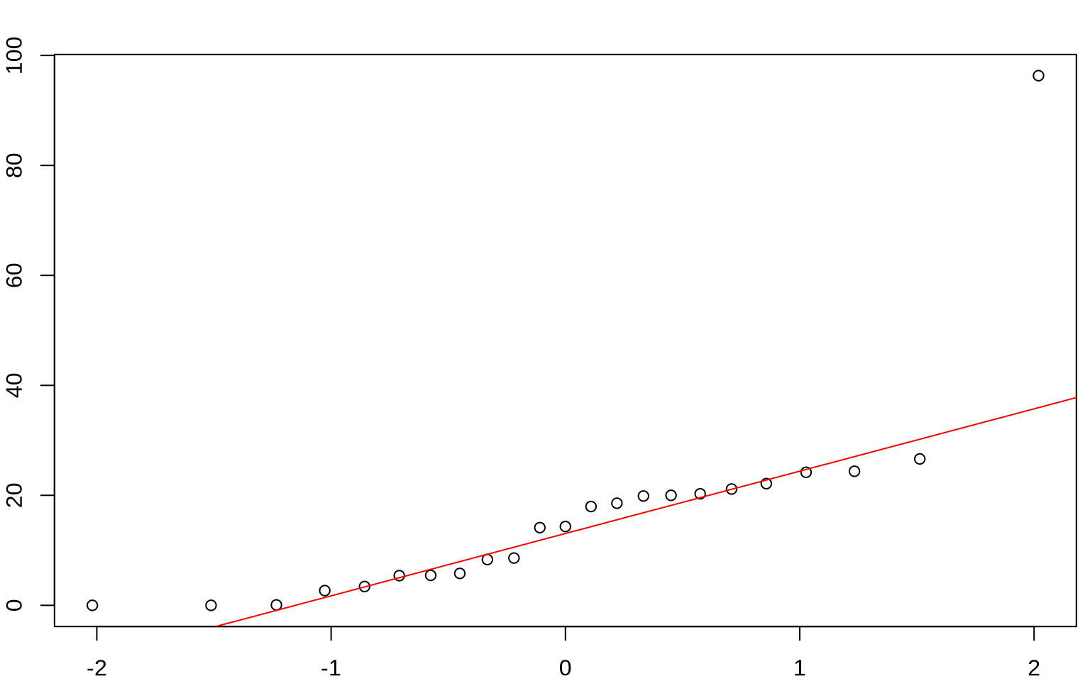
Bootstrap Estimates of Principal Components
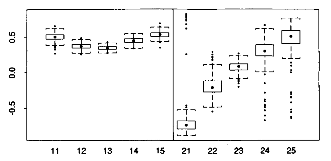
Bootstrap Estimates of Principal Components, \(\hat{\mathbf{v}}_1\) (left panel) and \(\hat{\mathbf{v}}_2\) (right panel) shows empirical distribution of the 200 bootstrap replications \(\hat{v}_{i k}^*\).
Verizon Data
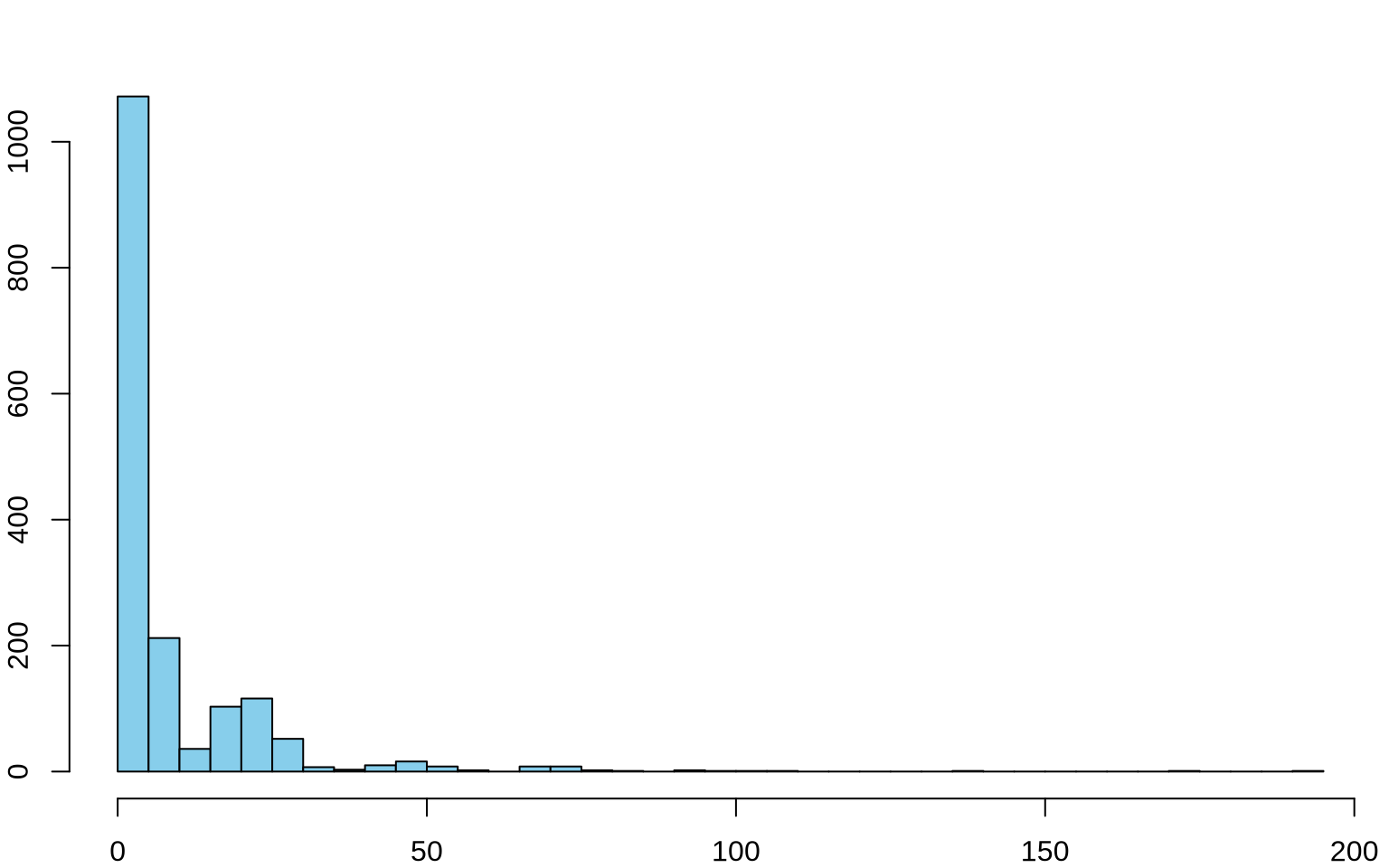
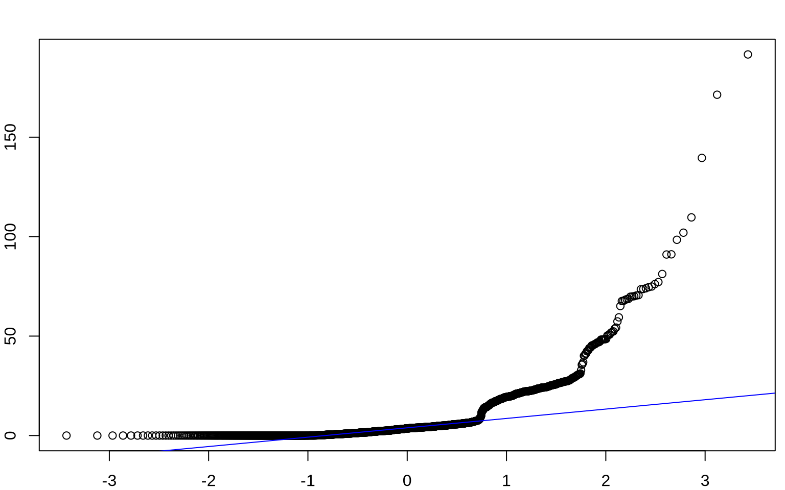
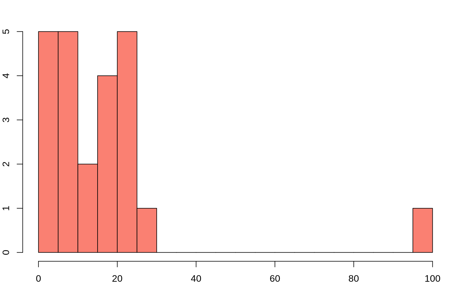
Permutation Test: Verizon Example
Code
# Calculate the observed difference in means
observed_diff <- mean(CLEC) - mean(ILEC)

set.seed(123)

# Function to perform permutation test
permutation_test <- function(data1, data2, num_permutations = 10000) {
  combined <- c(data1, data2)
  perm_diffs <- numeric(num_permutations)
  for (i in 1:num_permutations) {
    permuted <- sample(combined)
    perm_clec <- permuted[1:length(data1)]
    perm_ilec <- permuted[(length(data1) + 1):length(combined)]
    perm_diffs[i] <- mean(perm_clec) - mean(perm_ilec)
  }
  return(perm_diffs)
}

# Perform the permutation test
perm_diffs <- permutation_test(CLEC, ILEC)

# Calculate the p-value
p_value <- mean(abs(perm_diffs) >= abs(observed_diff))

# Plot the permutation distribution
perm_diffs_df <- data.frame(perm_diffs = perm_diffs)
ggplot(perm_diffs_df, aes(x = perm_diffs)) +
  geom_histogram(binwidth = 0.1) +
  geom_vline(aes(xintercept = observed_diff), color = "red", linetype = "dashed") +
  labs(x = "Difference in Means", y = "Frequency")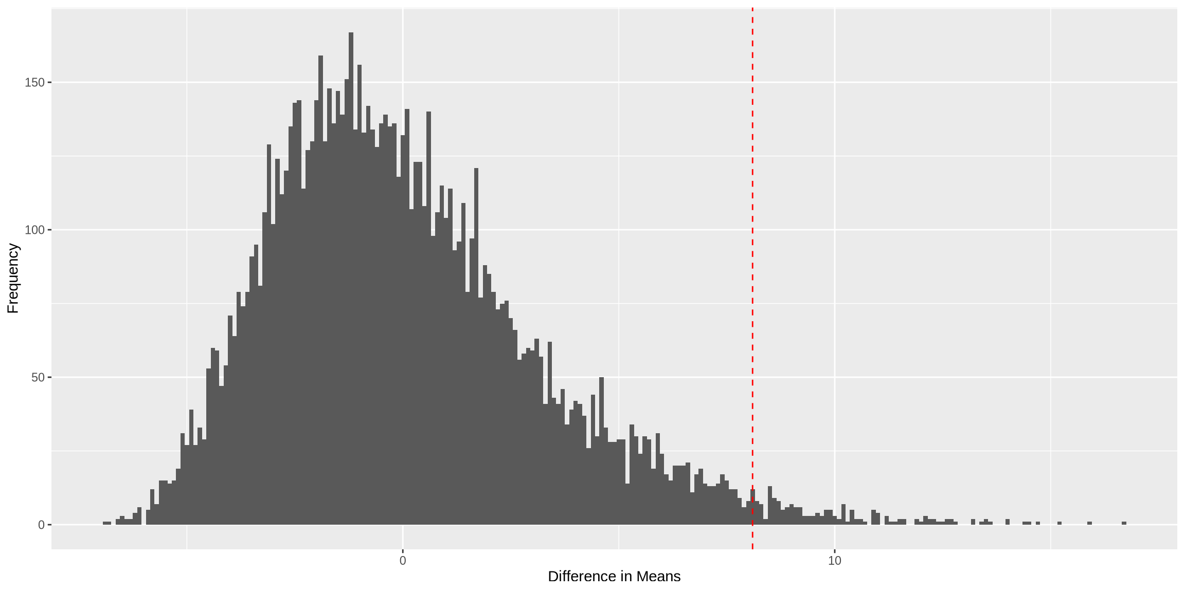
| Test | p-value |
|---|---|
| t-test | 0.0299 |
| Permutation | 0.0183 |