Linear algebra for data science

PSTAT 234 (Fall 2025)

Sang-Yun Oh

University of California, Santa Barbara

Matrix Multiplication: Elements of \(\boldsymbol{C}\)

Let \(\boldsymbol{C}\) be an \(m \times n\) matrix.

The \((i, j)\)-th element of the matrix product \(\boldsymbol{C}=\boldsymbol{A} \boldsymbol{B}\) is given by \[C_{i j}=A_{i\bullet} \cdot B_{\bullet j}\]

(Test scores example)

Matrix Multiplication: Rows of \(\boldsymbol{C}\)

Let \(\boldsymbol{C}\) be an \(m \times n\) matrix.

The \(i\)-th row of the matrix product \(\boldsymbol{C}=\boldsymbol{A} \boldsymbol{B}\) is given by \[C_{i \bullet}=A_{i\bullet} \cdot B\]

(Test scores example)

Matrix Multiplication: Columns of \(\boldsymbol{C}\)

Let \(\boldsymbol{C}\) be an \(m \times n\) matrix.

The \(j\)-th column of the matrix product \(\boldsymbol{C}=\boldsymbol{A} \boldsymbol{B}\) is given by

\[C_{\bullet j}=A \cdot B_{\bullet j}\]

(Test scores example)

Matrix Multiplication: \(\boldsymbol{C}=\boldsymbol{A} \boldsymbol{B}\)

Let \(\boldsymbol{C}\) be an \(m \times n\) matrix.

The matrix product \(\boldsymbol{C}=\boldsymbol{A} \boldsymbol{B}\) is given by \[C=\sum_{k=1}^K A_{\bullet k} \cdot B_{k \bullet}\]

(Test scores example)

Single Factor Representation of Data

  • Recall the IQ model for student test scores: i.e., \(\hat x_i = q_i v,\) \[\hat x_i = \begin{pmatrix} \hat x_{i1} & \hat x_{i2} & \cdots & \hat x_{i5} \end{pmatrix}',\ v = \begin{pmatrix} v_1 & v_2 & \cdots & v_5 \end{pmatrix}'\] where student \(i\)’s test scores \(\hat x_i\) is \(v\) scaled by \(q_i\).
  • Matrix form: for \(n\) students, \(q_i\)’s form a vector \(q = (q_1, q_2, \ldots, q_n)'\). \[ \hat X = \begin{pmatrix} \hat x_{11} & \hat x_{12} & \cdots & \hat x_{15} \\ \hat x_{21} & \hat x_{22} & \cdots & \hat x_{25} \\ \vdots \\ \hat x_{n1} & \hat x_{n2} & \cdots & \hat x_{n5} \end{pmatrix} = \begin{pmatrix} q_1 \\ q_2 \\ \vdots \\ q_n \end{pmatrix} \begin{pmatrix} v_1 & v_2 & \cdots & v_5 \end{pmatrix} \]
  • Individual characteristic (IQ) vector \(q\) and test characteristic vector \(v\) describe the data matrix \(\hat X\). Note that row \((\hat X)_{i\bullet}\) is \(\hat x_i'\).

library(bootstrap)
data(scor)

pc <- prcomp(scor, scale = FALSE, center = TRUE)  # PCA
eig <- eigen(cov(scor))   # Eigen decomposition of covariance matrix

# Compare PC loadings with eigenvectors
abs(eig$vectors) - abs(pc$rotation)
              PC1           PC2           PC3           PC4           PC5
mec  8.881784e-16 -1.110223e-16  2.553513e-15 -2.331468e-15 -3.608225e-16
vec  1.110223e-16  1.665335e-16  7.494005e-15 -3.774758e-15  9.159340e-16
alg -1.110223e-16 -3.885781e-16  8.049117e-16 -4.996004e-16  5.551115e-16
ana  0.000000e+00  8.881784e-16 -5.884182e-15  4.773959e-15  1.665335e-16
sta -1.110223e-16  3.330669e-16 -1.665335e-15  5.134781e-15 -2.775558e-17
# compare signs
sign(eig$vectors) * sign(pc$rotation)
    PC1 PC2 PC3 PC4 PC5
mec   1   1  -1   1  -1
vec   1   1  -1   1  -1
alg   1   1  -1   1  -1
ana   1   1  -1   1  -1
sta   1   1  -1   1  -1

Rank-\(k\) Approximation of Test Scores Data

Code
pc_approx_scor <- function(pc, num_pcs = 1) {
  Q = pc$x[,1:num_pcs]        # first PC scores
  V = pc$rotation[,1:num_pcs] # first PC loadings
  mu = pc$center              # variable means

  scor_hat = Q %*% t(V) + mu
  return(scor_hat)
}

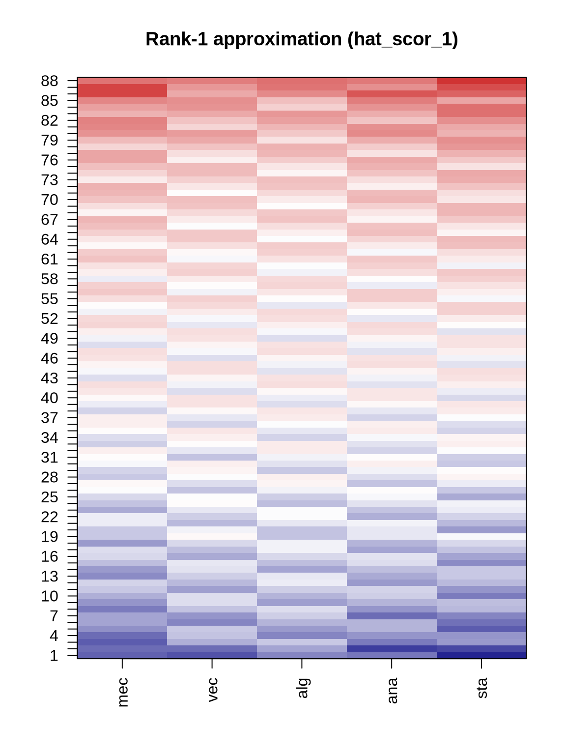
hat_scor_1 = pc_approx_scor(pc, num_pcs = 1)
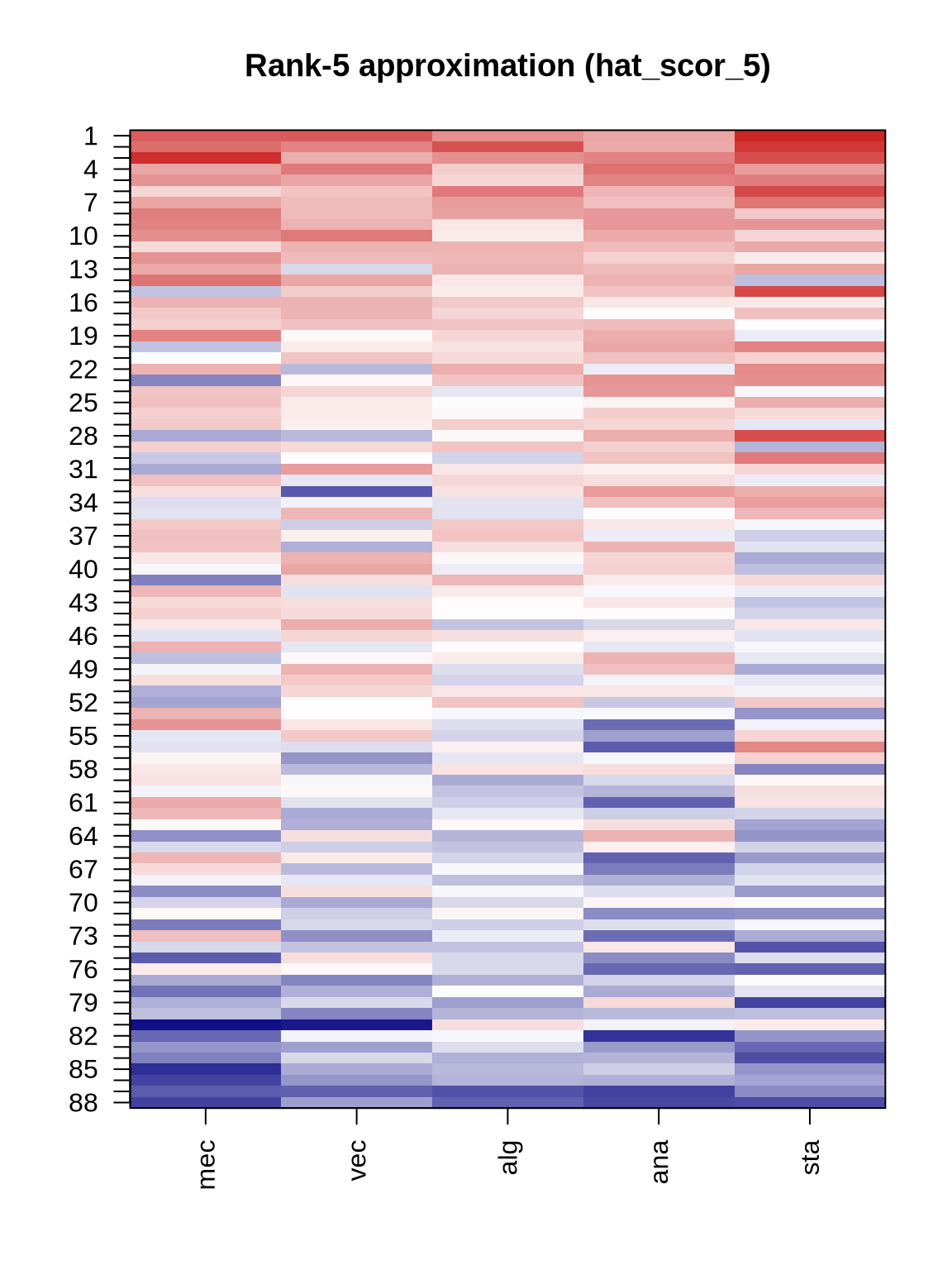
hat_scor_5 = pc_approx_scor(pc, num_pcs = 5)

# heatmaps: original scor vs rank-1 approximation
cols <- colorRampPalette(c("navy", "white", "firebrick3"))(100)
zmin <- min(c(as.matrix(scor), as.matrix(hat_scor_1), as.matrix(hat_scor_5)))
zmax <- max(c(as.matrix(scor), as.matrix(hat_scor_1), as.matrix(hat_scor_5)))

plot_heat <- function(mat, main = "") {
  m <- as.matrix(mat)
  image(1:ncol(m), 1:nrow(m), t(apply(m, 2, rev)),
        col = cols, axes = FALSE, xlab = "", ylab = "",
        main = main, zlim = c(zmin, zmax))
  axis(1, at = 1:ncol(m), labels = colnames(m), las = 2)
  axis(2, at = 1:nrow(m), labels = rev(rownames(m)), las = 2)
  box()
}
  
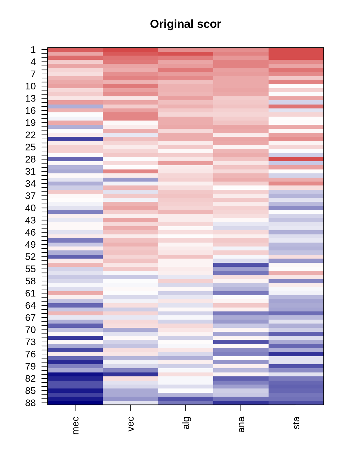
plot_heat(scor, "Original scor")
plot_heat(hat_scor_1, "Rank-1 approximation (hat_scor_1)")
plot_heat(hat_scor_5, "Rank-5 approximation (hat_scor_5)")

Original

Rank-1 Approximation

Rank-5 Approximation

Matrix Multiplication: Elements of \(\hat{X}\)

  • \(K\): number of latent features (PCs) (maximum \(K=5\))
  • \(Q\): matrix of size \(88 \times K\) individual features (\(Q = q\) when \(K=1\))
  • \(V\): matrix of size \(5 \times K\) test characteristics (\(V = v\) when \(K=1\)):
    \[ v_{jk} = (V)_{jk} = (V')_{kj}\]
  • For single factor model, i.e., \(K=1\), individual \(i\)’s \(j\)-th test score is
    \[ \hat X_{ij} = (q v')_{ij} = q_i\, v_j \]
  • For \(K=5\), student \(i\)’s \(j\)-th test score has following expression: \[ \hat X_{ij} = Q_{i\bullet} (V')_{\bullet j} = \sum_{k=1}^5 q_{ik}\, v_{jk} \]

Matrix Multiplication: Rows of \(\hat{X}\)

  • \(K\): number of latent features (PCs)
  • \(Q\): matrix of size \(88 \times K\) individual features (\(Q = q\) when \(K=1\))
  • \(V\): matrix of size \(5 \times K\) test characteristics (\(V = v\) when \(K=1\)):
    \[ v_{jk} = (V)_{jk} = (V')_{kj}\]
  • When \(K=1\), all test scores of student \(i\) has following expression: \[ \hat X_{i\bullet} = q_i v' \]
  • When \(K=5\), all test scores for student \(i\) has following expression: \[ \hat X_{i\bullet} = Q_{i\bullet} V' \]

Matrix Multiplication: Columns of \(\hat{X}\)

  • \(K\): number of latent features (PCs)
  • \(Q\): matrix of size \(88 \times K\) individual features (\(Q = q\) when \(K=1\))
  • \(V\): matrix of size \(5 \times K\) test characteristics (\(V = v\) when \(K=1\)):
    \[ v_{jk} = (V)_{jk} = (V')_{kj}\]
  • When \(K=1\), everyone’s scores of test \(j\) has following expression: \[ \hat X_{\bullet j} = q v_j \]

  • When \(K=5\), everyone’s scores of test \(j\) has following expression: \[ \hat X_{\bullet j} = Q (V')_{\bullet j} \]

Matrix Multiplication: \(\hat{X}\)

  • \(K\): number of latent features (PCs)
  • \(Q\): matrix of size \(88 \times K\) individual features (\(Q = q\) when \(K=1\))
  • \(V\): matrix of size \(5 \times K\) test characteristics (\(V = v\) when \(K=1\)):
    \[ v_{jk} = (V)_{jk} = (V')_{kj}\]
  • When \(K=1\), all scores of all tests has following expression: \[ \hat X = (Q)_{\bullet 1} (V')_{1 \bullet} = q v' \]

  • When \(K=5\), all scores of all tests has following expression: \[ \hat X = \sum_{k=1}^5 (Q)_{\bullet k} (V')_{k \bullet} \]

Matrix Factorization as Representation Learning

  • Many ways to factorize a data matrix \(X\) into product of two matrices \(W\) and \(Y\)
    • PCA: \(X \approx Q Y\), where \(Q\): orthogonal matrix of principal components, \(Y\): PC scores
    • ICA: \(X = W Y\), where \(W\): independent components, \(Y\): mixing coefficients
    • NMF: \(X \approx W H\), where \(W,H\): non-negative matrices
  • Different constraints on \(W\) and \(Y\) lead to different interpretations of the factors
  • Each can be viewed as representation learning technique that extract meaningful features from data
  • Choice of method depends on data characteristics and analysis goals

Non-negative Matrix Factorization

  • Assume data \(X\) is \(p\times n\) matrix of non-negative values

  • e.g., images, probabilities, counts, etc

  • NMF computes the following factorization:
    \[ \min_{W,H} \| X - WH \|_F\\ \text{ subject to } W\geq 0,\ H\geq 0, \] where \(W\) is \({p\times r}\) matrix and \(H\) is \({r\times n}\) matrix consist of non-negative values.

  • Each vectorized image is a column of \(X\)

NMF for Image Analysis

nmf-faces

NMF for Hyperspectral image analysis

nmf-hyper

NMF for Document Topic Discovery

nmf-topics

Representation Learning of Movie Ratings Data

Representing movie data as matrix factors

Interpretation of Matrix Factors

Interpretation of matrix factor subspaces

References