Linear algebra for data science, Part 2

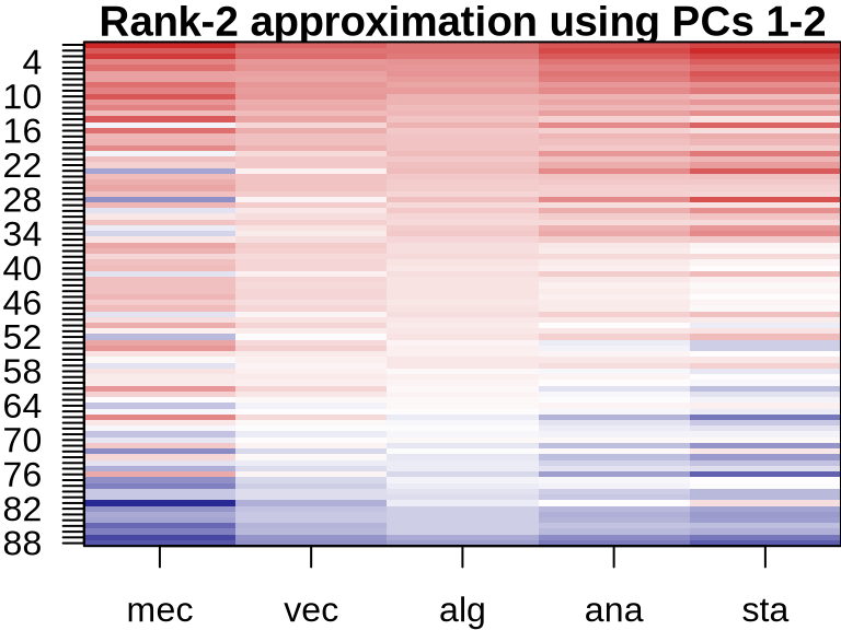
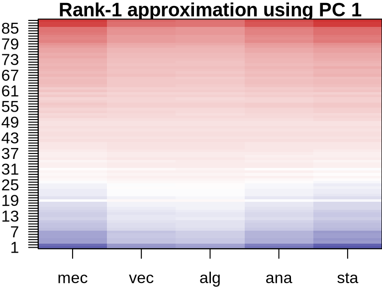
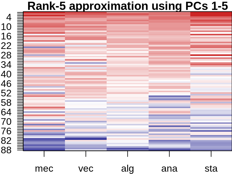
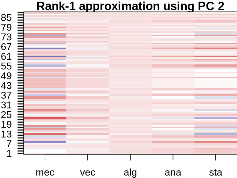
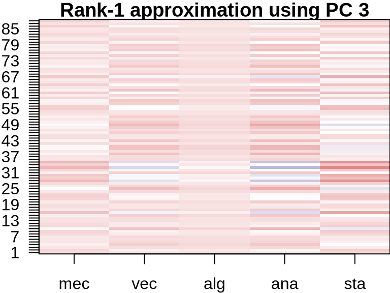
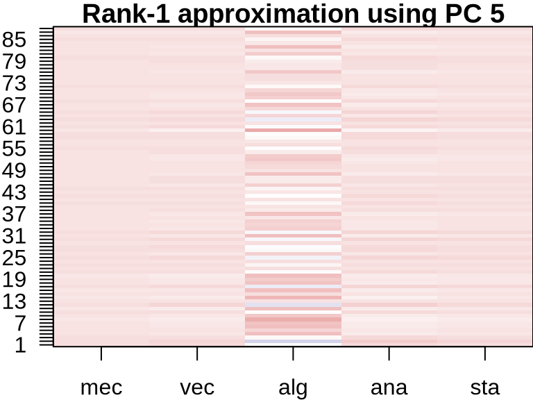
PCA: Visualizing Component Contributions

$\cdots + Q_{\bullet 5}(V_{\bullet 5})'$

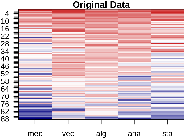
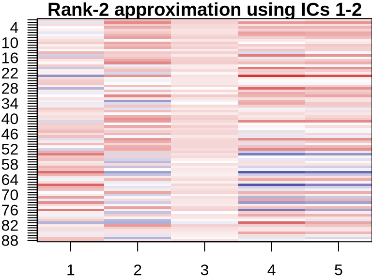
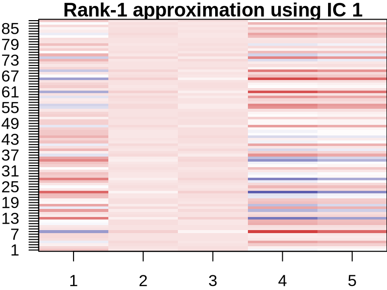
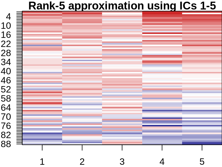
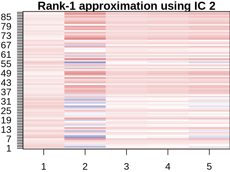
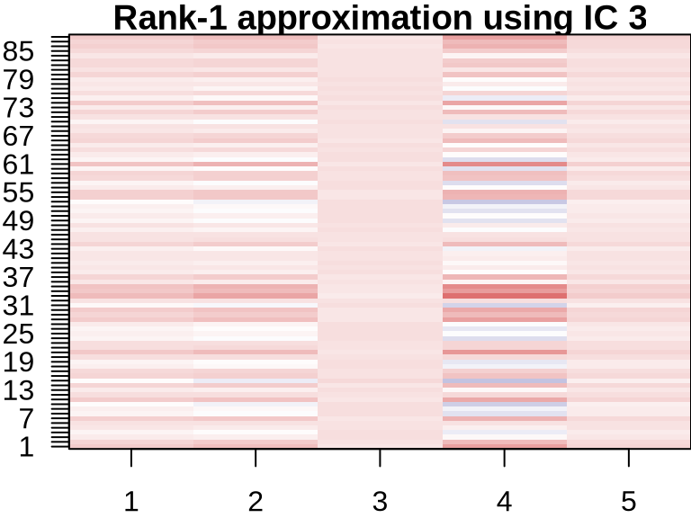
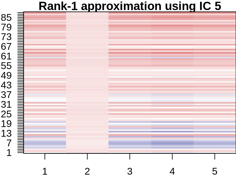
ICA: Visualizing Component Contributions

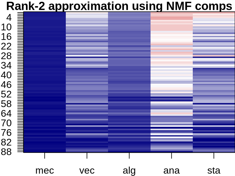
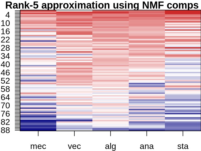
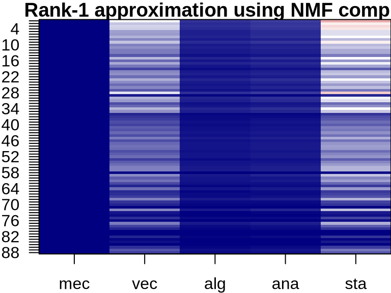
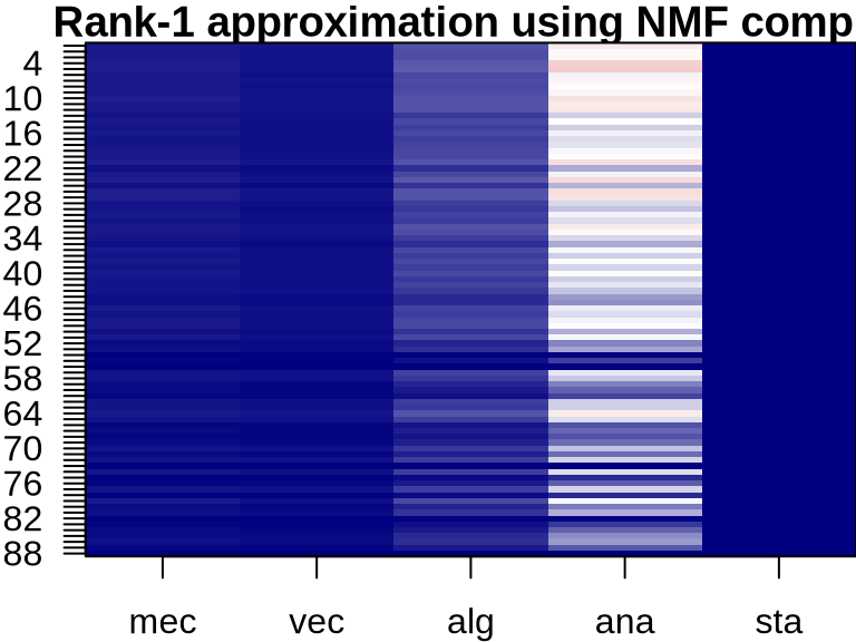
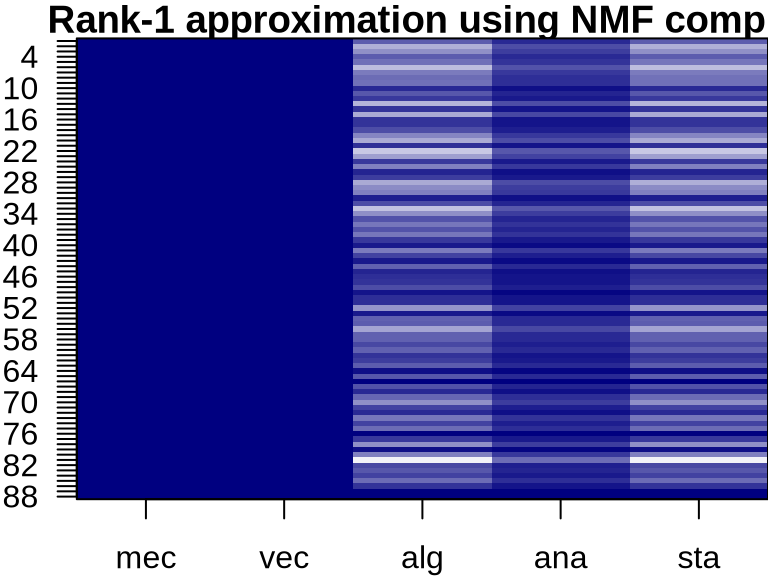
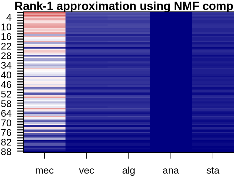
NMF: Visualizing Component Contributions

Comparison of PCA, ICA, and NMF Approximations

All are matrix factorization techniques that decompose data into components and scores
PCA components are orthogonal and capture maximum variance
ICA components are statistically independent and capture non-Gaussian structures
NMF components are non-negative and capture parts-based representations
Each method has different assumptions and is suitable for different types of data and analysis goals

Independent Components Analysis

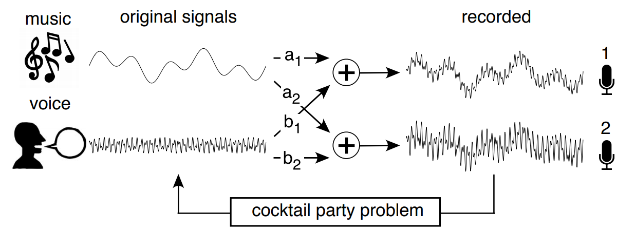
Blind source separation problem

Independent Components Analysis

$X$: Data matrix of size $\mathbb{R}^{n\times p}$

Independent Components Analysis (ICA): $ X = W Y $
- $W$: independent components
- $Y$: mixing coefficients
Independent components matrix $W$ (hopefully) represents underlying signals
Matrix $Y$ contain mixing coefficients

ICA vs PCA

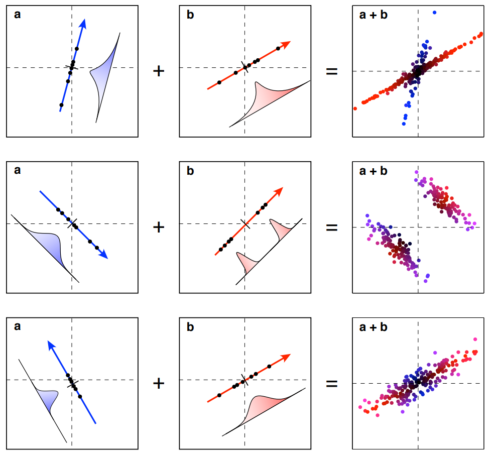
Hypothetical Simulation Data

ICA vs PCA

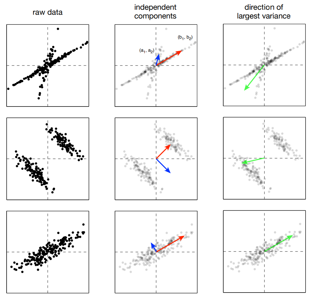
Partial ICA and PCA Results

ICA Identifiability

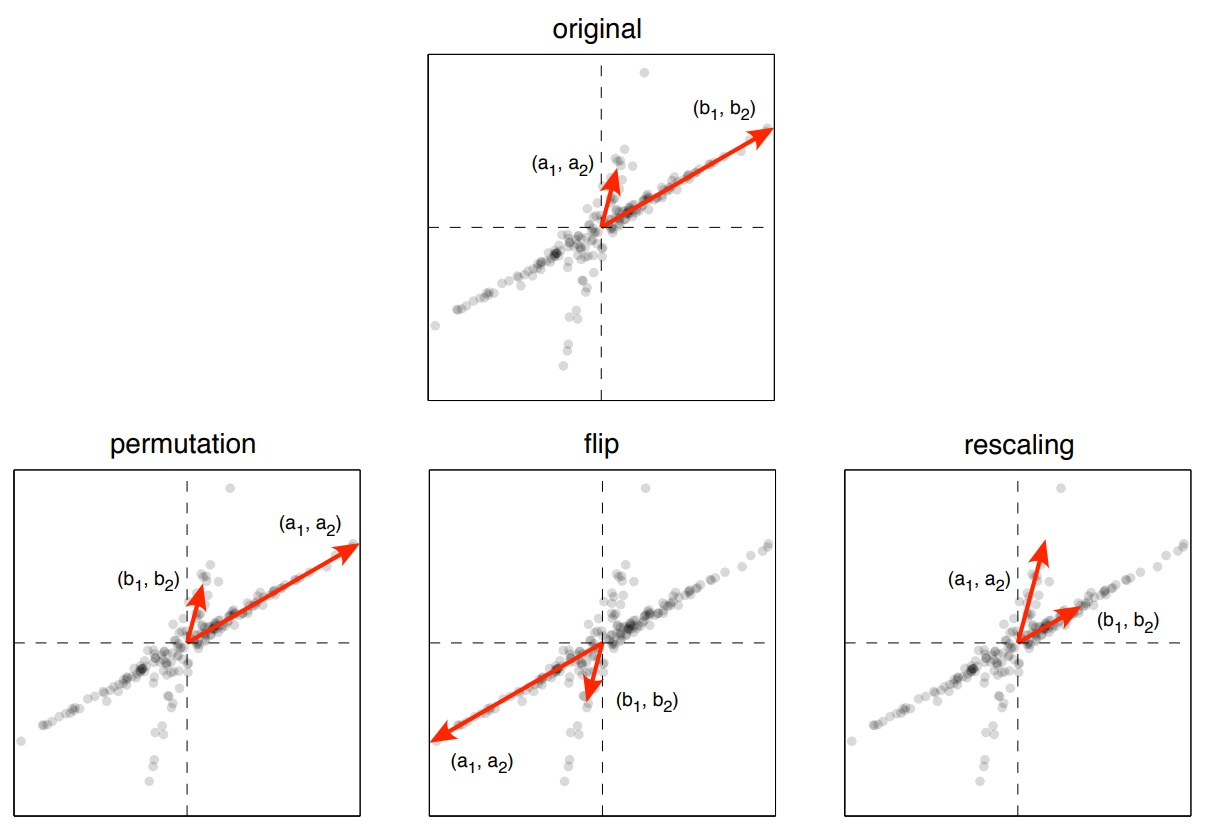
Identifiability

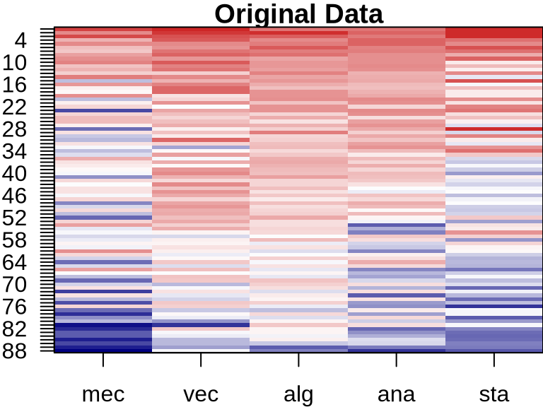
Eigenfaces: Data

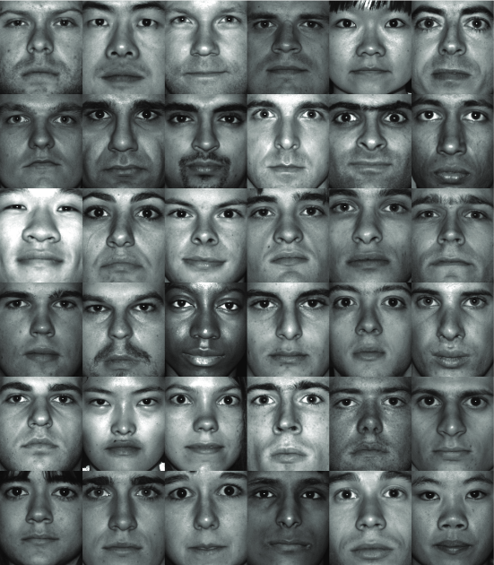
Eigenfaces example data (Brunton and Kutz 2019)

Various SVD forms

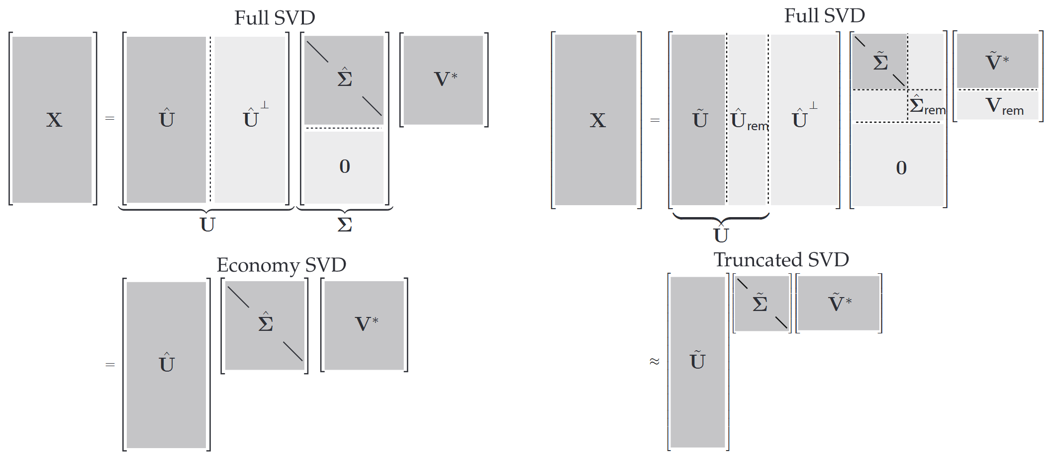
SVD forms (Brunton and Kutz 2019)

\[ \begin{aligned} X_\text{tr} \approx \hat X_\text{tr} &= U_\text{tr} \Sigma_\text{tr} V_\text{tr}^* = U_\text{tr} W_\text{tr}^* \\ X_\text{ts} \stackrel{\text{?}}{\approx} \hat X_\text{ts} &= U_\text{tr} (U_\text{tr}^* X_\text{ts}) \\ \end{aligned} \] where $U$, $V$, and $\Sigma$ are from SVD (hat or tilde variations), and $W = \Sigma V^*$.

Eigenfaces: SVD

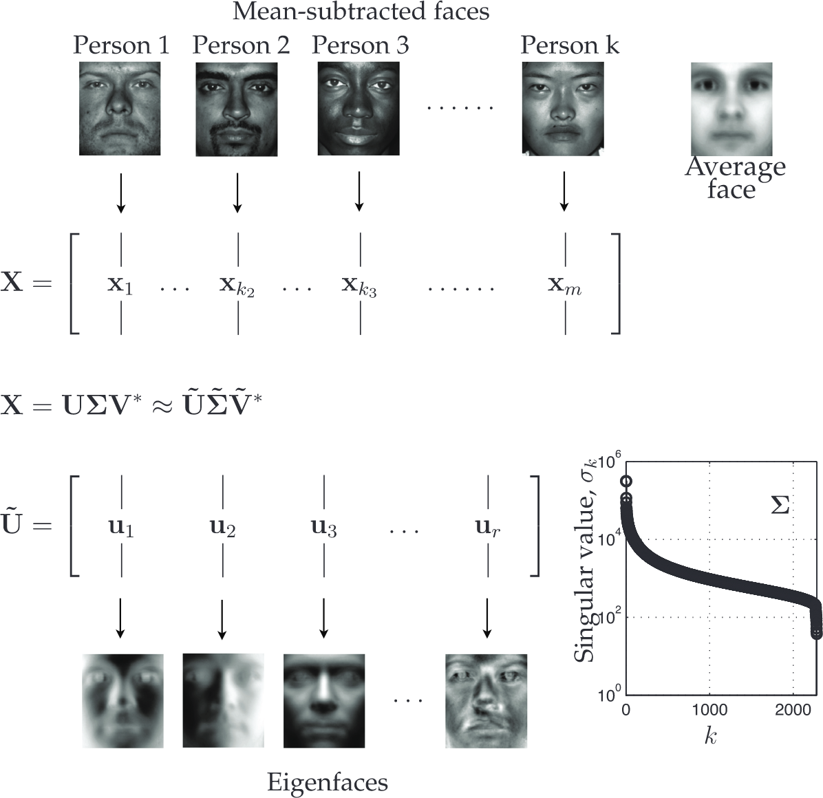
Eigenfaces and SVD (Brunton and Kutz 2019)

Eigenfaces: Reconstructing Test Image

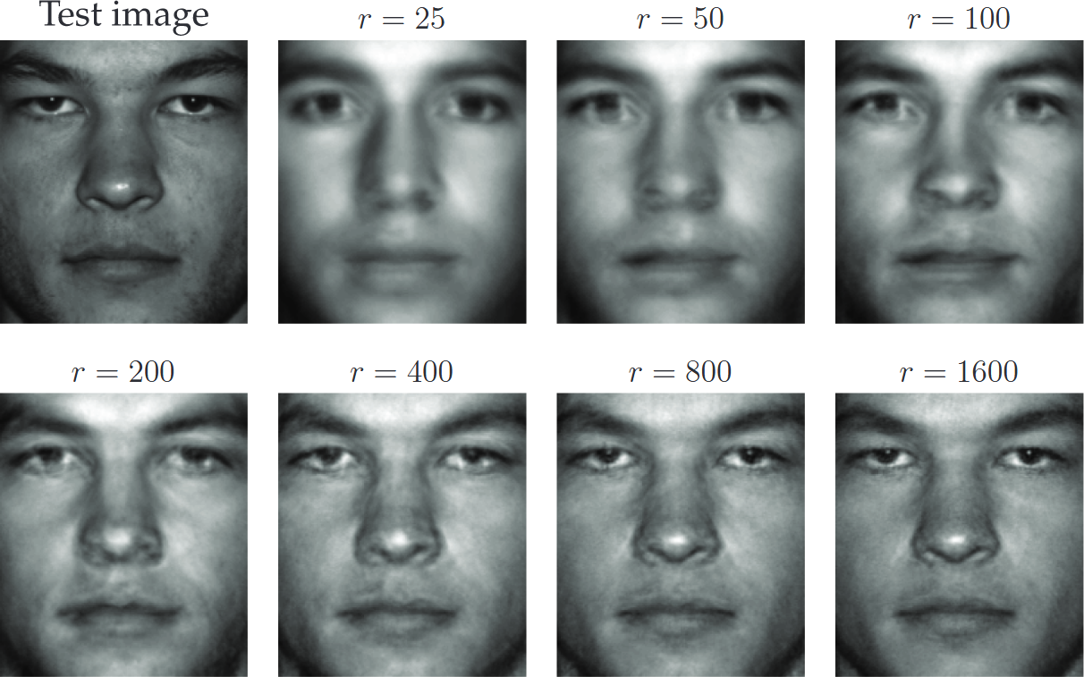
Face test image reconstruction (Brunton and Kutz 2019)

Eigenfaces: Reconstructing Test Image

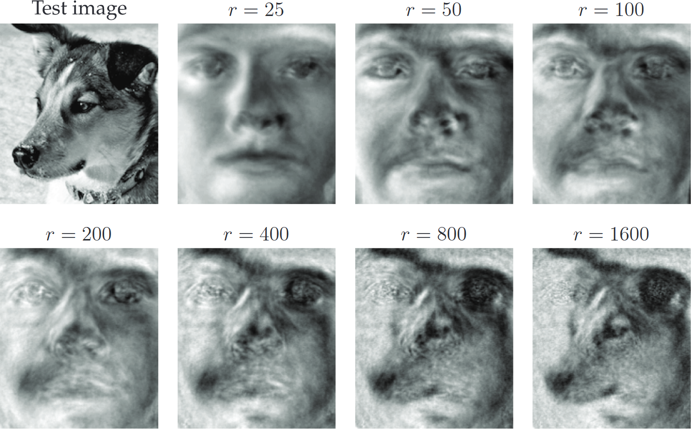
Dog test image reconstruction (Brunton and Kutz 2019)

Eigenfaces: Reconstructing Test Image

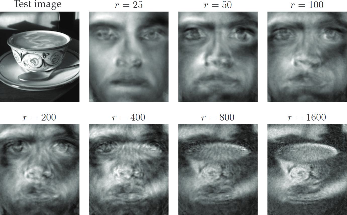
Cup test image reconstruction (Brunton and Kutz 2019)

Singular Value Decomposition (SVD) and

SVD is related to eigenvalue problem involving $\boldsymbol{X X}^*$ and $\boldsymbol{X}^* \boldsymbol{X}$:

\[ \begin{aligned} \boldsymbol{X X}^*&=\boldsymbol{U}\left[\begin{array}{c} \hat{\boldsymbol{\Sigma}} \\ \boldsymbol{0} \end{array}\right] \boldsymbol{V}^* \boldsymbol{V}\left[\begin{array}{ll} \hat{\boldsymbol{\Sigma}} & \boldsymbol{0} \end{array}\right] \boldsymbol{U}^*\\ &=\boldsymbol{U}\left[\begin{array}{cc} \hat{\boldsymbol{\Sigma}}^2 & \boldsymbol{0} \\ \boldsymbol{0} & \boldsymbol{0} \end{array}\right] \boldsymbol{U}^* \\ \end{aligned} \]

\[ \begin{aligned} \mathbf{X X}^* \mathbf{U}&=\mathbf{U}\left[\begin{array}{cc} \hat{\boldsymbol{\Sigma}}^2 & \mathbf{0} \\ \mathbf{0} & \mathbf{0} \end{array}\right] \\ \end{aligned} \]

Singular Value Decomposition (SVD) and

SVD is related to eigenvalue problem involving $\boldsymbol{X X}^*$ and $\boldsymbol{X}^* \boldsymbol{X}$:

\[ \begin{aligned} \boldsymbol{X}^* \boldsymbol{X}&=\boldsymbol{V}\left[\begin{array}{ll} \hat{\boldsymbol{\Sigma}} & \boldsymbol{0} \end{array}\right] \boldsymbol{U}^* \boldsymbol{U}\left[\begin{array}{c} \hat{\boldsymbol{\Sigma}} \\ \boldsymbol{0} \end{array}\right] \boldsymbol{V}^*\\ &=\boldsymbol{V} \hat{\boldsymbol{\Sigma}}^2 \boldsymbol{V}^* \end{aligned} \]

\[ \begin{aligned} \boldsymbol{X}^* \boldsymbol{X}&=\boldsymbol{V}\left[\begin{array}{ll} \hat{\boldsymbol{\Sigma}} & \boldsymbol{0} \end{array}\right] \boldsymbol{U}^* \boldsymbol{U}\left[\begin{array}{c} \hat{\boldsymbol{\Sigma}} \\ \boldsymbol{0} \end{array}\right] \boldsymbol{V}^*\\ &=\boldsymbol{V} \hat{\boldsymbol{\Sigma}}^2 \boldsymbol{V}^*\\ \mathbf{X}^* \mathbf{X} \mathbf{V}&=\mathbf{V} \hat{\mathbf{\Sigma}}^2 \end{aligned} \]

Linear Independence and Unique information

Orthogonal matrix $Q$: all columns are linearly independent to each other
If $Q$ is also orthnormal, $Q$ is orthogonal and each column is of length 1
Therefore, if $Q$ is orthonormal, \[ QQ^T = Q^TQ = I \]

Vector spaces or Subspaces

Vector Space (Subspace) in $\Re^m$

A non-empty set $\mathcal{S} \subseteq \Re^m$ is called a vector space in $\Re^m$ (or a subspace of $\Re^m$ ) if both of the following conditions are satisfied:

If $\boldsymbol{x} \in \mathcal{S}$ and $\boldsymbol{y} \in \mathcal{S}$, then $\boldsymbol{x}+\boldsymbol{y} \in \mathcal{S}$. In other words, $\mathcal{S}$ is closed under vector addition.
If $\boldsymbol{x} \in \mathcal{S}$, then $\alpha \boldsymbol{x} \in \mathcal{S}$ for all $\alpha \in \Re^1$. In other words, $\mathcal{S}$ is closed under scalar multiplication.

The above two criteria can be combined to say that a non-empty set $\mathcal{S} \subseteq \Re^m$ is a subspace if $\boldsymbol{x} + \alpha \boldsymbol{y} \in \mathcal{S}$ for every $\boldsymbol{x}, \boldsymbol{y} \in \mathcal{S}$ and every $\alpha\in\Re^1$.

Consider vectors as elements from data
Subspaces are the sets of vectors that can be added or multiplied by scalars without leaving the set.
Subspaces represent the space in which linear operations can yield results that are still in the space.

Null Spaces of a Matrix

Null Space of a Matrix $\boldsymbol{A}$

Let $\boldsymbol{A}$ be an $m \times n$ matrix in $\Re^{m \times n}$. The null space of $\boldsymbol{A}$ is defined as the set

\[ \mathcal{N}(\boldsymbol{A})=\left\{\boldsymbol{x} \in \Re^n: \boldsymbol{A} \boldsymbol{x}=\mathbf{0}\right\}. \]

Any member of the set $\mathcal{N}(\boldsymbol{A})$ is an $n \times 1$ vector, so $\mathcal{N}(\boldsymbol{A})$ is a subset of $\Re^n$.

Saying that $\boldsymbol{x} \in \mathcal{N}(\boldsymbol{A})$ is the same as saying $\boldsymbol{x}$ satisfies $\boldsymbol{A} \boldsymbol{x}=\mathbf{0}$.

Left Null Space of a Matrix $\boldsymbol{A}$

Let $\boldsymbol{A}$ be an $m \times n$ matrix in $\Re^{m \times n}$. The left null space of $\boldsymbol{A}$ is defined as the set

\[ \mathcal{N}\left(\boldsymbol{A}^{\prime}\right)=\left\{\boldsymbol{x} \in \Re^m: \boldsymbol{A}^{\prime} \boldsymbol{x}=\mathbf{0}\right\} \]

is called the . Any member of the set $\mathcal{N}\left(\boldsymbol{A}^{\prime}\right)$ is an $m \times 1$ vector, so $\mathcal{N}\left(\boldsymbol{A}^{\prime}\right)$ is a subset of $\Re^m$.

Equivalently, $\mathcal{N}\left(\boldsymbol{A}^{\prime}\right)=\{\boldsymbol{x} \in$ $\left.\Re^m: \boldsymbol{x}^{\prime} \boldsymbol{A}=\mathbf{0}^{\prime}\right\}$.

Fundamental Subspaces

The four fundamental subspaces of a matrix $A$ are

Column space $\mathcal{C}(A)$
Null space $\mathcal{N}(A)$
Row space $\mathcal{C}(A^T)$
Left null space $\mathcal{N}(A^T)$

Linear Independence and Dependence

Linear Independence

Let $\mathcal{A}=\left\{\boldsymbol{a}_1, a_2, \ldots, a_n\right\}$ be a finite set of vectors with each $\boldsymbol{a}_i \in$ $\Re^m$. The set $\mathcal{A}$ is said to be linearly independent if the following condition holds: whenever $x_i$ ’s are real numbers such that

\[ x_1 \boldsymbol{a}_1+x_2 \boldsymbol{a}_2+\cdots+x_n \boldsymbol{a}_n=\mathbf{0} \]

we have $x_1=x_2=\cdots=x_n=0$. On the other hand, whenever there exist real numbers $x_1, x_2, \ldots, x_n$, not all zero, such that $x_1 \boldsymbol{a}_1+x_2 \boldsymbol{a}_2+\cdots+x_n \boldsymbol{a}_n=\mathbf{0}$, we say that $\mathcal{A}$ is linearly dependent.

\[ \mathcal{A}_1=\left\{\left[\begin{array}{l} 1 \\ 0 \end{array}\right],\left[\begin{array}{l} 0 \\ 1 \end{array}\right]\right\} \quad \text { and } \quad \mathcal{A}_2=\left\{\left[\begin{array}{l} 1 \\ 0 \end{array}\right],\left[\begin{array}{l} 0 \\ 1 \end{array}\right],\left[\begin{array}{l} 2 \\ 3 \end{array}\right]\right\} . \]

$\mathcal{A}_1$ is clearly a linearly independent set
$\mathcal{A}_2$ is clearly a linearly dependent set.
“Linearly independent set of vectors” or “linearly dependent set of vectors.”

Linear Independence and Dependence in Data

In data analysis, we often deal with sets of vectors representing observations or features.
Linear independence among these vectors implies that each vector contributes unique information that cannot be derived from the others.
Conversely, linear dependence indicates redundancy, where some vectors can be expressed as combinations of others.
Understanding the linear independence or dependence of data vectors is crucial for dimensionality reduction, feature selection, and ensuring the robustness of statistical models.

References

Brunton, Steven L., and J. Nathan Kutz. 2019. Data-Driven Science and Engineering. Cambridge University Press. https://doi.org/10.1017/9781108380690.