Mathematical Programming/Optimization, Part 1

Linear Algebra and Data Science

Often, data science problems have equivalent optimization problems.
For example, linear regression, principal component analysis (PCA), and support vector machines (SVMs)
Solutions are the best ones in terms of these optimization problems.
Solutions can be characterized using linear algebra concepts.
Computational algorithms are implemented with linear algebra libraries.
Connection between linear algebra and optimization is crucial for developing effective data science methods.
Linear algebra: language and tools to represent and manipulate data.

Linear Algebra and Data Science: OLS example

Many problems in data science can be formulated as optimization problems: e.g., if data, $(y_i, x_i)$ where $i=1,\ldots,n$, is given, OLS finds the best-fitting line

\[ \min _{\beta_0, \beta_1} \sum_{i=1}^n\left(y_i-\beta_0-\beta_1 x_i\right)^2 = \min _\beta\|\mathbf{y}-\mathbf{X} \boldsymbol{\beta}\|^2 \]

How can the analytical solution given by \[ \hat{\beta}=\left(\mathbf{X}^T \mathbf{X}\right)^{-1} \mathbf{X}^T \mathbf{y} \] be obtained/characterized?

Observations of OLS Problem

\[ \min _{\beta_0, \beta_1} \sum_{i=1}^n\left(y_i-\beta_0-\beta_1 x_i\right)^2 = \min _\beta\|\mathbf{y}-\mathbf{X} \boldsymbol{\beta}\|_2^2 \]

Objective yields a scalar value (SSE).
Objective is a function of parameters $\boldsymbol{\beta} = (\beta_0,\ \beta_1)'$.
No constraints on parameters (unconstrained problem).
What if norm in objective changes to
- $\| v \|_1 = \sum_{i=1}^n \left|v_i\right|$
- $\| v \|_\infty = \max_{i=1,\ldots,n} \left|v_i\right|$
- $\| v \|_p = \left(\sum_{i=1}^n \left|v_i\right|^p\right)^{1/p}$

Observations of OLS Problem

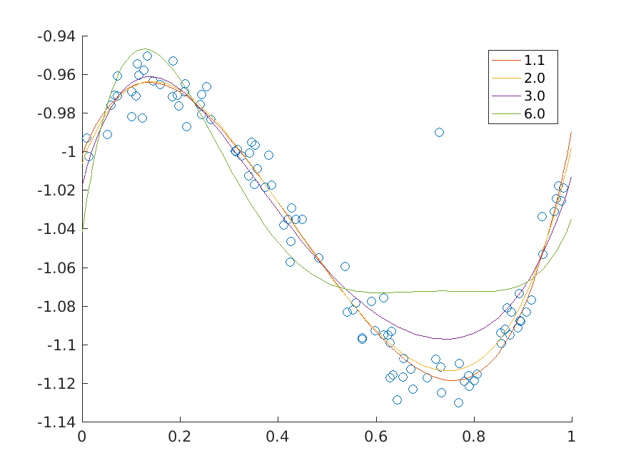
$p$-norm minimizing fits of a polynomial of degree at most 5 to the data for various values of $p$.

Principal Component Analysis (PCA) as Optimization

For centered data matrix $X\in \mathbb{R}^{n \times p}$ ($n$ observations and $p$ variables).

First PC loading vector $v_1$ can be obtained by solving,

\[ \begin{aligned} \max _{v_1} &\quad v_1^T X^T X v_1,\\ \text{subject to} &\quad v_1^T v_1=1 \quad \text{(length constraint)} \end{aligned} \]

Second PC loading vector $v_2$ can be obtained by solving, \[ \begin{aligned} \max _{v_2} &\quad v_2^T X^T X v_2,\\ \text{subject to} &\quad v_2^T v_2=1 \quad \text{(length constraint)} \\ &\quad v_2^T v_1=0 \quad \text{(orthogonality constraint)} \end{aligned} \]

PCA as Optimization (contd.)

The $k$-th PC loading vector $v_k$ can be obtained by solving, \[ \begin{aligned} \max _{v_k} &\quad v_k^T X^T X v_k, & \\ \text{subject to} &\quad v_k^T v_k=1 \quad \text{(length constraint)} \\ &\quad v_j^T v_k=0, j=1, \ldots, k-1 \\ &\quad \text{(orthogonality constraint)} \end{aligned} \]

Connection to SVD of $X = U\Sigma V^T$:

\[ n S=X' X=\left(U \Sigma V'\right)'\left(U \Sigma V'\right)=V \Sigma^2 V' \]

Thus, $v_k$ is the $k$-th right singular vector of $X$ corresponding to the $k$-th largest singular value $\sigma_k$.

General Mathematical Programming/Optimization

Mathematical Programming/Optimization

A mathematical programming/optimization problem has the form

\[ \begin{array}{ll} \operatorname{minimize}_x & f_0(x) \\ \operatorname{subject to} & f_i(x) \leq b_i, \quad i=1, \ldots, m \end{array} \]

Optimization variable: $x=\left(x_1, \ldots, x_n\right)$
Objective function: $f_0: \mathbf{R}^n \rightarrow \mathbf{R}$
Constraints: $f_i: \mathbf{R}^n \rightarrow \mathbf{R}$, $i=1, \ldots, m$
Constraint limits/bounds: $b_1, \ldots, b_m$

A vector $x^{\star}$ is optimal for the problem, if it has the smallest objective value among all vectors that satisfy the constraints.

That is, for any $z$ with $f_1(z) \leq b_1, \ldots, f_m(z) \leq b_m$, we have $f_0(z) \geq f_0\left(x^{\star}\right)$.

Linear Programming Problem

Linear Programming Problem

Optimization problem is called a linear program if the objective and constraint functions $f_0, \ldots, f_m$ are linear, i.e., satisfy

\[ f_i(\alpha x+\beta y)=\alpha f_i(x)+\beta f_i(y) \]

for all $x, y \in \mathbf{R}^n$ and all $\alpha, \beta \in \mathbf{R}$.

Exercise: does $f(x) = a x + b$ qualify as linear? (assume $x$ is scalar)

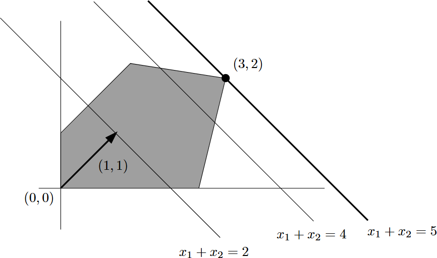
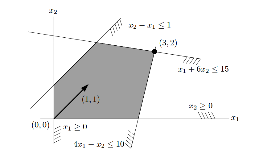
Example: Linear Programming Problem

\[ \begin{aligned} \text{maximize}_{\left(x_1, x_2\right) \in \mathbb{R}^2}\quad & x_1+x_2\\ \operatorname{subject to}\quad & x_1 \geq 0,\, x_2 \geq 0 \\ & x_2-x_1 \leq 1 \\ & x_1+6 x_2 \leq 15 \\ & 4 x_1-x_2 \leq 10 \end{aligned} \]

Food	Carrot, Raw	White Cabbage, Raw	Cucumber, Pickled	Required per dish
Vitamin A (mg/kg)	35	0.5	0.5	0.5 mg
Vitamin C (mg/kg)	60	300	10	15 mg
Dietary Fiber (g/kg)	30	20	10	4 g
price ($/kg)	0.75	0.5	0.15	-

Example: Linear Programming Problem

At what minimum price per dish can the requirements of the Office of Nutrition Inspection be satisfied?

\[ \begin{array}{ll} \text { minimize } & 0.75 x_1+0.5 x_2+0.15 x_3 \\ \text { subject to } & x_1 \geq 0,\, x_2 \geq 0,\, x_3 \geq 0 \\ & 35 x_1+0.5 x_2+0.5 x_3 \geq 0.5 \\ & 60 x_1+300 x_2+10 x_3 \geq 15 \\ & 30 x_1+20 x_2+10 x_3 \geq 4 \end{array} \]

LP Exception Cases

When a linear program has no feasible solutions, it is called infeasible.
When a linear program has feasible solutions but can be arbitrarily large in value, it is called unbounded.
When a linear program has feasible solutions and an optimal solution, but the optimal solution is not unique, it is called degenerate.

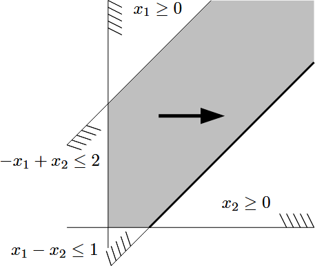
LP Exception Cases: Unboundedness

\[ \begin{array}{ll} \operatorname{maximize} & x_1 \\ \text { subject to } & x_1-x_2 \leq 1 \\ & -x_1+x_2 \leq 2 \\ & x_1, x_2 \geq 0 \end{array} \]

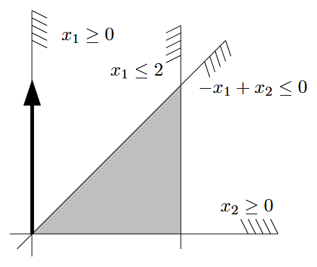
LP Exception Cases: Degeneracy

\[ \begin{array}{lcl} \operatorname{minimize} & x_2 & \\ \text { subject to } & -x_1+x_2 \leq 0 \\ & x_1 \leq 2 \\ & x_1, x_2 \geq 0 \end{array} \]

Standard Form of LP

Standard Form of LP

A linear program can be written in the following standard form:

\[ \begin{array}{ll} \text { Maximize the value of } & \mathbf{c}^T \mathbf{x} \\ \text { among all vectors } \mathbf{x} \in \mathbb{R}^n \text { satisfying } & A \mathbf{x} \leq \mathbf{b}, \end{array} \]

where $A$ is a given $m \times n$ real matrix and $\mathbf{c} \in \mathbb{R}^n, \mathbf{b} \in \mathbb{R}^m$ are given vectors. Here inequality holds for two vectors of equal length if and only if it holds componentwise.

Any vector $\mathbf{x} \in \mathbb{R}^n$ satisfying all constraints of a given linear program is a feasible solution. Each $\mathbf{x}^* \in \mathbb{R}^n$ that gives the maximum possible value of $\mathbf{c}^T \mathbf{x}$ among all feasible $\mathbf{x}$ is called an optimal solution, or optimum for short.

General Form of LP

Rewriting the standard form of LP explicitly,

\[ \begin{aligned} &\begin{array}{ll} \text { maximize the value of } & \mathbf{c}^T \mathbf{x} \\ \text { among all vectors } \mathbf{x} \in \mathbb{R}^n \text { satisfying } & A \mathbf{x} \leq \mathbf{b}, \end{array}\\ \quad \\ = &\begin{array}{ll} \text { maximize } & \mathbf{c}^T \mathbf{x} =c_1 x_1+c_2 x_2+\cdots+c_n x_n \\ \text { subject to } & a_{11} x_1+a_{12} x_2+\cdots+a_{1 n} x_n \leq b_1 \\ & a_{21} x_1+a_{22} x_2+\cdots+a_{2 n} x_n \leq b_2 \\ & \vdots \\ & a_{m 1} x_1+a_{m 2} x_2+\cdots+a_{m n} x_n \leq b_m \end{array} \end{aligned} \]

Convex Optimization Problem

Linear Programming Problem

Optimization problem is called a linear program if the objective and constraint functions $f_0, \ldots, f_m$ are linear, i.e., satisfy

\[ f_i(\alpha x+\beta y)=\alpha f_i(x)+\beta f_i(y) \]

for all $x, y \in \mathbf{R}^n$ and all $\alpha, \beta \in \mathbf{R}$.

Convex Optimization Problem

A convex optimization problem is one in which the objective and constraint functions are convex, which means they satisfy the following inequality:

\[ f_i(\alpha x+\beta y) \leq \alpha f_i(x)+\beta f_i(y) \]

for all $x, y \in \mathbf{R}^n$ and all $\alpha, \beta \in \mathbf{R}$ with $\alpha+\beta=1, \alpha \geq 0, \beta \geq 0$.