Mathematical Programming/Optimization, Part 2
Convex Optimization

PSTAT 234 (Fall 2025)

Sang-Yun Oh

University of California, Santa Barbara

Example Optimization Problem: Internet Ads

Problem formulation for Internet Ads

Suppose we are an advertising agency and want to optimize ad scheduling over \(T\) time slots.

  • Ads/advertisers: \(a=1, \ldots, A\) (total of \(A\) ads)
  • Timeslots: \(t=1, \ldots, T\) (up to \(T\) time slots)
  • Site visitors: \(v_t\) in time slot \(t\)
  • Ads displayed: \(d_{at} \geq 0\) is ad \(a\) displayed in period \(t\).

Our constraints are

  • At most \(v_t\) displays: \(\sum_a d_{at} \leq v_t\)
  • At least \(c_a\) displays: \(\sum_t d_{at} \geq c_a\) (by contract).
  • Our goal is to choose \(d_{at}\).

Clicks and revenue

  • Number of clicks: \(k_{at}\) on ad \(a\) in period \(t\).
  • Click model: \(k_{at} = p_{at}d_{at}\), where
  • Click probability: \(p_{at} \in [0,1]\) is for ad \(a\) in time \(t\).
  • Ad revenue: \(s_a\) from ad \(a\), where one click pays \(r_a\), up to budget \(b_a\).

\[ s_a = \min \left\{ r_a \sum_t k_{at}, b_a\right\}, \]

  • What do we want to optimize?
  • What shape is \(s_a\) as a function of \(d_{at}\)?

Ad optimization

We choose displays \(d_{at}\) to maximize revenue, i.e., we solve

\[ \begin{array}{ll} \operatorname{maximize}_{d_{at}} & \sum_a s_a \\ \mbox{subject to} & d_{at} \geq 0 \quad \text{(non-negative displays)} \\ & \sum_a d_{at} \leq v_t \quad \text{(limited visitors to site)} \\ & \sum_t d_{at} \geq c_a \quad \text{(contractual obligations)} \end{array} \]

Generate synthetic data

Generate synthetic data for ad optimization problem:

Code
import numpy as np

np.random.seed(30)
A = 5  # Number of ads
T = 24  # Number of time slots
SCALE = 10000

# Budget for ads: b_a
b = np.random.lognormal(mean=8, size=(A,)) + 10000
b = 1000 * np.round(b / 1000)

# Probability of click: p_{at} ∈ R^{AxT}
P = 0.05 * np.random.uniform(size=(A, T))

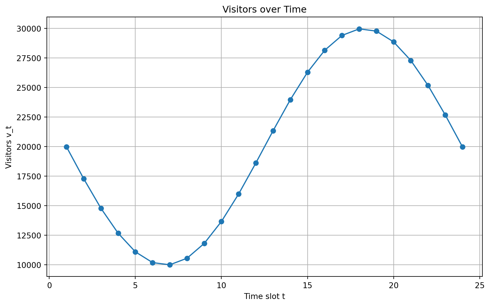
# Visitors over time: v_t ∈ R^T
v = np.sin(np.linspace(-2 * np.pi / 2, 2 * np.pi - 2 * np.pi / 2, T)) * SCALE
v += -np.min(v) + SCALE

# Contracted impressions: c_a ∈ R^A
c = np.random.uniform(size=A)
c *= 0.9 * v.sum() / c.sum()
c = 1000 * np.round(c / 1000)

# Revenue per click: r_a ∈ R^A
r = np.random.lognormal(mean=0.0, sigma=0.5, size=A)
ad 0 1 2 3 4
b (budget) 11000 24000 11000 15000 13000
c (contracted impr) 88000 101000 148000 52000 43000
r (revenue per click) 1.164 0.741 2.37 1.12 1.104

View data

Code
# Visualize visitors over time and show ad parameters
# Line chart for visitors v_t
plt.figure(figsize=(10, 6))
plt.plot(np.arange(1, T + 1), v, marker='o')
plt.title('Visitors over Time')
plt.xlabel('Time slot t')
plt.ylabel('Visitors v_t')
plt.grid(True)
plt.show()

Solve Optimization Problem

Code
# Form and solve the optimal advertising problem (maximize sum_a s_a)
import cvxpy as cp

D = cp.Variable((A, T))  # D_{a,t}
s = []
for a in range(A):
    clicks_a = cp.sum(cp.multiply(P[a, :], D[a, :]))  # ∑_t p_{a,t} d_{a,t}
    s.append(cp.minimum(r[a] * clicks_a, b[a]))       # s_a = min{ r_a * clicks_a, b_a }

prob = cp.Problem(
    cp.Maximize(cp.sum(s)),
    [
        D >= 0,                              # non-negative displays
        cp.sum(D, axis=0) <= v,              # ∑_a d_{a,t} ≤ v_t
        cp.sum(D, axis=1) >= c,              # ∑_t d_{a,t} ≥ c_a
    ],
)
prob.solve()
25962.688502001343

Check Constraints

Print if all constraints are satisfied:

Code
# Check constraints
displays = D.value
print("Check non-negative displays (D >= 0):", np.all(displays >= 0))
print("Check limited visitors to site (∑_a d_{a,t} ≤ v):", np.all(displays.sum(axis=0) <= v + 1e-5))
print("Check contractual obligations (∑_t d_{a,t} ≥ c):", np.all(displays.sum(axis=1) >= c - 1e-5))
print("Check if total revenue is within budgets:", all(
    r[a] * (P[a, :] @ displays[a, :]) <= b[a] + 1e-5 for a in range(A)
))
Check non-negative displays (D >= 0): True
Check limited visitors to site (∑_a d_{a,t} ≤ v): True
Check contractual obligations (∑_t d_{a,t} ≥ c): True
Check if total revenue is within budgets: True

Print total revenue achieved:

Code
# Calculate total revenue
total_revenue = prob.value
print("Total Revenue Achieved: $", round(total_revenue, 2))
Total Revenue Achieved: $ 25962.69

Optimization Algorithms: Gradient Descent

Direction of Function Decrease

Find \(x^*\) that minimize function \(f(x)\): \[ x^* = \arg\min_x f(x). \]

  • Starting at \(x=a\), is minimum to left or right?

  • Starting at \(x=a\), does \(f(x)\) decreases to left or right?

  • Repeatedly decrease \(f(x)\) by adjusting \(x\)

  • When \(f(x)\) stops decreasing (\(x\) converges to a point), stop

  • How to determine the direction of function decrease?

Univariate Convex Function

Convex Function

Differentiable convex function \(g(x)\) satisfies \[g(x) \geq g(a) + g'(a)(x-a),\] for any valid \(x\) and \(a\)

Convex function \(g(x) = (x-2)^2 + 1\) and its tangent line at \(x=a\)

Descent Direction

Convex Function

Differentiable convex function \(g(x)\) satisfies \[g(x) \geq g(a) + g'(a)(x-a),\] for any valid \(x\) and \(a\)

  • Starting at point \(a\), find \(b\) decreases \(f\): i.e.,
    \[f(a) - f(b) \geq 0\]

  • For a convex function \(f\), show that \(b\) satisfies \[f'(a)(b-a) \leq 0\]

Example: Univariate Quadratic Function

Objective function: \(f(x) = (x+1)^2\) and \(x\in\mathbb{R}\)

  • Satisfying \(f^{\prime}(a)(b-a)\leq 0\)

    • Case 1: if slope \(f'(a)<0\), we need \(b>a\): i.e. move right.
    • Case 2: if slope is \(f'(a)>0\), we need \(b<a\): i.e. move left
    • Case 3: if slope is \(f'(a)=0\), we are at the minimum
  • \(b \leftarrow a - f'(a)\) is a possibility, but could overshoot!

  • How big of a step? A small enough \(\alpha\) (step size) works: \[b \leftarrow a - \alpha\cdot f'(a)\]

Example 1: Univariate Quadratic Function

Code
def f(x): return (x+1)**2
def fprime(x): return 2*(x+1)

def find_minimum_1(func, slope, a = 2, step=0.1, max_iter=1000):
    
    for i in range(0, max_iter):
        
        # find next target point
        b = a - step*slope(a)
        
        # set target point as the new starting point
        a = b
    
    return b

x = np.linspace(-10, 10, num=1000)
xstar = find_minimum_1(f, fprime)

print('  xstar  = %f, f(xstar) = %f' % (xstar, f(xstar)))
  xstar  = -1.000000, f(xstar) = 0.000000

Function \(f(x) = (x+1)^2\) and its minimum point

Example 2: Univariate Quadratic Function

Code
def g(x): return (x-3.2)**2 - x + 2.3
def gprime(x): return 2*(x-3.2) - 1

x = np.linspace(-3, 8, num=1000)
xstar = find_minimum_1(g, gprime)

print('  xstar  = %f, g(xstar) = %f' % (xstar, g(xstar)))
  xstar  = 3.700000, g(xstar) = -1.150000

Function \(g(x) = (x-3.2)^2 - x + 2.3\) and its minimum point

Improving Optimization Algorithm

def find_minimum_2(func, slope, x0 = 2, rate=0.1, message=False):

    assert(rate > 0 and rate < 1)

    c = 0
    for i in range(0, 1000):

        # find next target point 
        x1 = x0 - rate*slope(x0)
        
        if np.isclose(x1, x0, rtol=1e-5):
            if message:
                print('converged in %d iterations' % c)
            return x1
        
        if func(x1) < func(x0): # func decreased
            x0 = x1
            c += 1
        else:                   # func did not decrease
            rate *= rate        # reduce step size
    
    print('warning: algorithm did not converge')
    
    return x1

xstar = find_minimum_2(g, gprime, message=True) ## less number of loops
g(xstar)
converged in 41 iterations
-1.1499999790850541

Complexity vs. Running time

Algorithm complexity and running times are different concepts:

%timeit -n10 -r10 find_minimum_1(g, gprime) ## faster running time

%timeit -n10 -r10 find_minimum_2(g, gprime) ## slower running time
152 µs ± 52.5 µs per loop (mean ± std. dev. of 10 runs, 10 loops each)
991 µs ± 42.3 µs per loop (mean ± std. dev. of 10 runs, 10 loops each)

Directional Derivative and Gradient

Directional Derivative and Gradient

Let \(f: D \rightarrow \mathbb{R}\) where \(D \subseteq \mathbb{R}^d\), let \(\mathbf{x}_0 \in D\) be an interior point of \(D\) and let \(\mathbf{v} \in \mathbb{R}^d\) be a vector. Assume that \(f\) is continuously differentiable at \(\mathbf{x}_0\). Then the directional derivative of \(f\) at \(\mathbf{x}_0\) in the direction \(\mathbf{v}\) is given by

\[ \frac{\partial f\left(\mathbf{x}_0\right)}{\partial \mathbf{v}}=\nabla f\left(\mathbf{x}_0\right)^T \mathbf{v} \]

Contour plot of \(f(x, y) = (x-1)^2 + (y-2)^2\)

Multivariate Convex Function

First-Order Convexity Condition

Let \(f: D \rightarrow \mathbb{R}\) be continuously differentiable, where \(D \subseteq \mathbb{R}^d\) is convex. Then \(f\) is convex over \(D\) if and only if

\[ f(\mathbf{y}) \geq f(\mathbf{x})+\nabla f(\mathbf{x})^T(\mathbf{y}-\mathbf{x}), \quad \forall \mathbf{x}, \mathbf{y} \in D \]

Note that the right-hand side is the linear approximation to \(f\) at \(\mathbf{x}\) from Taylor’s Theorem without the remainder.

Descent Direction and Directional Derivative

Let \(f: \mathbb{R}^d \rightarrow \mathbb{R}\) be continuously differentiable at \(\mathbf{x}_0\). A vector \(\mathbf{v}\) is a descent direction for \(f\) at \(\mathbf{x}_0\) if

\[ \frac{\partial f\left(\mathbf{x}_0\right)}{\partial \mathbf{v}}=\nabla f\left(\mathbf{x}_0\right)^T \mathbf{v}<0 \]

that is, if the directional derivative of \(f\) at \(\mathbf{x}_0\) in the direction \(\mathbf{v}\) is negative.

Gradient Descent Algorithm

Direction of Steepest Descent

Let \(f: \mathbb{R}^d \rightarrow \mathbb{R}\) be continuously differentiable at \(\mathbf{x}_0\). For any unit vector \(\mathbf{v} \in \mathbb{R}^d\),

\[ \frac{\partial f\left(\mathbf{x}_0\right)}{\partial \mathbf{v}} \geq \frac{\partial f\left(\mathbf{x}_0\right)}{\partial \mathbf{v}^*} \]

where

\[ \mathbf{v}^*=-\frac{\nabla f\left(\mathbf{x}_0\right)}{\left\|\nabla f\left(\mathbf{x}_0\right)\right\|} \]

Gradient Descent Algorithm

Each iteration of gradient descent takes a step in the direction of the negative of the gradient:

\[ \mathbf{x}^{t+1}=\mathbf{x}^t-\alpha_t \nabla f\left(\mathbf{x}^t\right), \quad t=0,1,2 \ldots \]

for a sequence of step sizes \(\alpha_t>0\). The algorithm is initialized with an initial guess \(\mathbf{x}^0\).

Example: Lasso Regression

The lasso can be written in Lagrangian (unconstrained) form as:

\[ \operatorname{minimize}_{\boldsymbol{\beta}} \quad \frac{1}{2}\|\mathbf{y} - \mathbf{X}\boldsymbol{\beta}\|_2^2 + \lambda \|\boldsymbol{\beta}\|_1 \]

where \(\mathbf{y} \in \mathbb{R}^n\) is response, \(\mathbf{X} \in \mathbb{R}^{n \times p}\) is design matrix, \(\boldsymbol{\beta} \in \mathbb{R}^p\) are coefficients, and \(\lambda \geq 0\) is regularization parameter.

In constrained form, \[ \begin{array}{ll} \operatorname{minimize}_{\boldsymbol{\beta}} & \frac{1}{2}\|\mathbf{y} - \mathbf{X}\boldsymbol{\beta}\|_2^2 \\ \text{subject to} & \|\boldsymbol{\beta}\|_1 \leq s \end{array}, \]

where \(s \geq 0\) controls the amount of regularization.

Example: Lasso Regression Feasible Region

Image: Introduction to Statistical Learning in Python

Other Types of Optimization Problems

  • Mixed Integer Programming (MIP): some variables constrained to be integers.
  • Quadratic Programming (QP): objective function is quadratic, constraints linear.
  • Second-Order Cone Programming (SOCP): constraints include second-order (quadratic) cones
  • Semidefinite Programming (SDP): constraints include positive semidefinite matrices.
  • Exponential and Power Cone Programming: constraints include exponential or power cones.

Libraries and Types of Optimization Problems

LP QP SOCP SDP EXP POW MIP
CBC X X
CLARABEL X X X X X X
COPT X X X X X X**
DAQP X X
GLOP X
GLPK X
GLPK_MI X X
OSQP X X
PIQP X X
PROXQP X X
PDLP X
QOCO X X X
CPLEX X X X X
NAG X x X
LP QP SOCP SDP EXP POW MIP
ECOS X X X X
GUROBI X X X X
MOSEK X X X X X X X**
MPAX X X
CUCLARABEL X X X X X
CUOPT X X*
CVXOPT X X X X
SDPA *** X X X X
SCS X X X X X X
SCIP X X X X
XPRESS X X X X
SCIPY X X*
HiGHS X X X*

When installed, these libraries can be interfaced with Python via CVXPY.