Covariance Matrix
- Covariance matrix is defined as $$ \Sigma=E(\boldsymbol{X}-\boldsymbol{\mu})(\boldsymbol{X}-\boldsymbol{\mu})^{\prime}=\left(\sigma_{i j}\right), $$
- Sample covariance matrix is $$ \mathbf{S}=\frac{1}{n} \sum_{i=1}^{n}\left(\boldsymbol{X}_{i}-\overline{\boldsymbol{X}}\right)\left(\boldsymbol{X}_{i}-\overline{\boldsymbol{X}}\right)^{\prime}, $$
- Other types of covariance estimates
Covariance Matrices in Practice
- Stocks: $p=4300+$ companies and 20 days per month
Relationship between stocks (volatility structure)
- Genomics: $p\approx 20000$ genes and 100s of subjects
Co-expression of genes (gene relevance network)
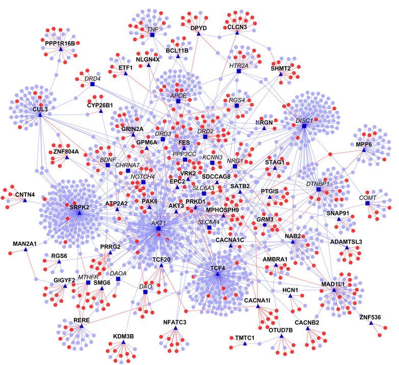
Shows protein-protein interaction network. Source: https://doi.org/10.1038/npjschz.2016.12
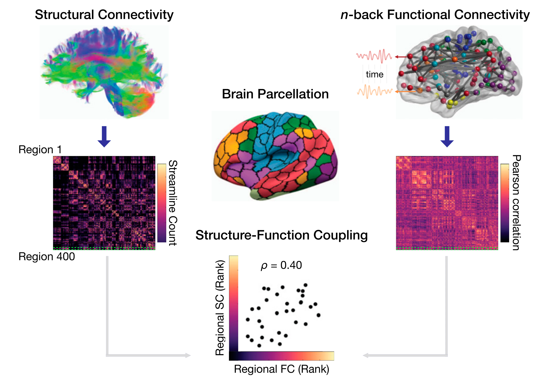
- Neuroimaging: $p=90000$ voxels (or hundreds of aggregated ROIs) and thousands of time points
Functional connectivity network
- Ecology: $p=23$ environmental variables and $n=12$ locations
Community abundance (Warton 2008)
Data are often high dimensional
Other Covariance Matrix Uses
- Markowitz Portfolio Problem (encodes market volatility)
- Regression (OLS)
$$ \widehat{\beta}_{\text {OLS}}=\left(\boldsymbol{X}^{\prime} \boldsymbol{X}\right)^{-1} \boldsymbol{X}^{\prime} \boldsymbol{Y} $$ - Canonical Correlation Analysis (CCA): associations among two sets of variables (examples)
- Input to clustering algorithm
- Inverse of $\Sigma$ often needed but doesn't exist in high dimensional setting
Mathematical Properties
- Matrix $\Sigma$ is symmetric
- All eigenvalues are nonnegative
- Nonnegative definite
- If singular, dimensionality can be reduced (assuming enough data is used)
Difficulty with Estimation of Covariance Matrices
- High dimensionality: $O(p^2)$ parameters grows faster than available samples ($n \ll p$)
- Sample deficiency: $\mathbf{S}$ is singular when $p>n$; poorly conditioned when $p$ close to $n$
- Eigenvalue distortion: extreme spread, noisy small eigenvalues (Marchenko–Pastur effects)
- Computational burden: forming/storing $\mathbf{S}$ is $O(p^2)$ memory, eigendecompositions $O(p^3)$
- Stability: high sensitivity to outliers, heavy tails, regime shifts, and nonstationarity
- Spurious correlations: many pairwise correlations appear significant by chance
- Missing data and asynchronous sampling (finance, genomics) complicate estimation
- Interpretability: dense estimates hinder structural insight (networks, factor structure)
- Downstream impact: inversion instability propagates to regression, portfolio optimization, CCA
Regularized Estimation
- Eigenvalue structure (Ledoit-Wolf, condition number)
- Sparsity pattern (graphical models)
- Structural assumptions (banding, tapering, low-rank)
All stabilize estimates (bias variance trade off)
Eigen-structure changes
- Eigenvector regularization (sparse PCA, SVD, etc)
- Ledoit-Wolf Estimator (Ledoit and Wolf, 2004) $$ \widehat{\mathbf{\Sigma}}=\alpha I+(1-\alpha) \mathbf{S} $$
Condition number regularization (Won et al., 2009)
$$ \begin{array}{ll} \operatorname{maximize} & l(\Sigma) \\ \text { subject to } & \operatorname{cond}(\Sigma) \leq \kappa_{\max }, \end{array} $$
where $l(\Sigma)$ is the Gaussian Likelihood
- Ridge regression: $\min_\beta \|Y - X\beta\|^2 +\gamma\|\beta\|_2^2$ $$ \widehat{\beta}_{\text {Ridge}}=\left(X^{\prime} X + \gamma I\right)^{-1} X^{\prime} Y $$
Sparsity Assumption (Graphical Model)
- $\mathbf{\Omega}=\mathbf{\Sigma}^{-1}$ appear in many situations
- $\mathbf{\Omega}$ can be regularized directly
- Assume $\boldsymbol{X}_{1}, \ldots, \boldsymbol{X}_{n} \sim N_{p}(\boldsymbol{0}, \boldsymbol{\Sigma})$ and $$ L(\boldsymbol{\Sigma})=\frac{1}{(2 \pi)^{n p / 2}|\boldsymbol{\Sigma}|^{n / 2}} \exp \left\{-\frac{1}{2} \sum_{i=1}^{n} \boldsymbol{X}_{i}^{\prime} \boldsymbol{\Sigma}^{-1} \boldsymbol{X}_{i}\right\} . $$
- Compute $\boldsymbol{\Omega}$: $$ \ell_{P}(\boldsymbol{\Omega})=\log |\boldsymbol{\Omega}|-\operatorname{tr}(\mathbf{S} \boldsymbol{\Omega})-\lambda\|\boldsymbol{\Omega}\|_{1}, $$
Reference: High‐Dimensional Covariance Estimation by Mohsen Pourahmadi
Multivariate Gaussian
The Setup: Partitioning the Vectors and Matrices
Let $x$ be a $D$-dimensional Gaussian random vector with mean $\mu$ and covariance $\Sigma$. We partition $x$ into two disjoint subsets, $x_a$ and $x_b$ (where we want to find the distribution of $x_a$ given $x_b$).
$$ x = \begin{bmatrix} x_a \\ x_b \end{bmatrix}, \quad \mu = \begin{bmatrix} \mu_a \\ \mu_b \end{bmatrix} $$
The joint distribution is defined as $p(x) = \\mathcal{N}(x | \mu, \Sigma)$.
1. In Terms of the Covariance Matrix ($\Sigma$)
We partition the covariance matrix $\Sigma$ to correspond with $x_a$ and $x_b$:
$$ \Sigma = \begin{bmatrix} \Sigma_{aa} & \Sigma_{ab} \\ \Sigma_{ba} & \Sigma_{bb} \end{bmatrix} $$
The conditional distribution $p(x_a | x_b)$ is also a Gaussian distribution $\mathcal{N}(x_a | \mu_{a|b}, \Sigma_{a|b})$.
The Conditional Mean
The mean of $x_a$ is adjusted by the deviation of $x_b$ from its mean, scaled by the correlation between the two:
$$ \mu_{a|b} = \mu_a + \Sigma_{ab}\Sigma_{bb}^{-1}(x_b - \mu_b) $$
The Conditional Covariance
The uncertainty in $x_a$ is reduced by the knowledge of $x_b$. This is mathematically represented by the Schur Complement of $\Sigma_{bb}$ in $\Sigma$:
$$ \Sigma_{a|b} = \Sigma_{aa} - \Sigma_{ab}\Sigma_{bb}^{-1}\Sigma_{ba} $$
Note: Calculating the conditional distribution using the covariance matrix requires computing the inverse of $\Sigma_{bb}$. If $x_b$ is high-dimensional, this is computationally expensive.
2. In Terms of the Precision Matrix ($\Omega$)
The Precision matrix (also called the information matrix) is the inverse of the covariance matrix: $\Omega = \Sigma^{-1}$. We partition $\Omega$ similarly:
$$ \Omega = \begin{bmatrix} \Omega_{aa} & \Omega_{ab} \\ \Omega_{ba} & \Omega_{bb} \end{bmatrix} $$
Note that because the inverse of a block matrix involves complex interactions between blocks, $\Omega_{aa}$ is not simply $\Sigma_{aa}^{-1}$.
When expressing the conditional distribution $p(x_a | x_b)$ using the precision matrix, the formulas usually become simpler and computationally more efficient, specifically for the covariance.
The Conditional Mean
$$ \mu_{a|b} = \mu_a - \Omega_{aa}^{-1}\Omega_{ab}(x_b - \mu_b) $$
The Conditional Covariance
Here is the elegant property of the precision matrix: The conditional precision is simply the corresponding block of the joint precision matrix. Therefore, the conditional covariance is just the inverse of that block:
$$ \Sigma_{a|b} = \Omega_{aa}^{-1} $$
Summary Comparison
| Parameter | Using Covariance Matrix ($\Sigma$) | Using Precision Matrix ($\Omega$) |
|---|---|---|
| Conditional Mean ($\mu_{a \mid b}$) | $\mu_a + \Sigma_{ab}\Sigma_{bb}^{-1}(x_b - \mu_b)$ | $\mu_a - \Omega_{aa}^{-1}\Omega_{ab}(x_b - \mu_b)$ |
| Conditional Covariance ($\Sigma_{a \mid b}$) | $\Sigma_{aa} - \Sigma_{ab}\Sigma_{bb}^{-1}\Sigma_{ba}$ | $\Omega_{aa}^{-1}$ |
Key Insight:
- Marginalization is easy with the Covariance matrix (you just take the sub-block $\Sigma_{aa}$).
- Conditioning is easy with the Precision matrix (you just take the sub-block $\Omega_{aa}$ and invert it).
- Zeros in the Covariance matrix imply marginal independence.
- Zeros in the Precision matrix imply conditional independence (essential for Gaussian Markov Random Fields).
Numerical Experiments
import pandas as pd
import numpy as np

store = pd.HDFStore('data/yfinance-data-store.h5')
logret = store['logret'].dropna().head(100)
Sample Covariance Matrix
$$ \mathbf{S}=\frac{1}{n} \sum_{i=1}^{n}\left(\boldsymbol{X}_{i}-\overline{\boldsymbol{X}}\right)\left(\boldsymbol{X}_{i}-\overline{\boldsymbol{X}}\right)^{\prime}, $$
- MLE of covariance matrix for Gaussian data
- Singular in high dimensional setting: Zero eigenvalues
- When $p>n$, other covariance estimates are needed
import sklearn.covariance as skcov
import sklearn.model_selection as sksel
import numpy.linalg as npl

cov_sample = skcov.empirical_covariance(logret)
Ledoit-Wolf Estimator
$$ \Sigma_{\text {LW}}=(1-\alpha) \mathbf{S}+\alpha \frac{\operatorname{Tr} \mathbf{S}}{p} \text { I } $$
- Ledoit and Wolf, 2004 (documentation page)
- Weighted average between sample covariance and identity (times average eigenvalue)
cov_lw, shrinkage_lw = skcov.ledoit_wolf(logret)
shrinkage_lw
0.19241305589502752
- Large eigenvalues decrease
- Zero eigenvalues increase (not sigular)
Graphical Model
# !pip install bokeh==2.4.1
# !pip install networkx
# !pip install robust-selection
edge_model = skcov.GraphicalLassoCV(n_refinements=2)
edge_model.fit(logret.head(30))
omega = edge_model.precision_.copy()
cov_ggm = npl.inv(edge_model.precision_)
/opt/conda/lib/python3.11/site-packages/numpy/core/_methods.py:173: RuntimeWarning: invalid value encountered in subtract
  x = asanyarray(arr - arrmean)
from bokeh.io import show, output_file, output_notebook
from bokeh.models import (BoxSelectTool, Circle, EdgesAndLinkedNodes,
                          HoverTool, MultiLine, NodesAndLinkedEdges,
                          Plot, Range1d, TapTool, LabelSet,
                          ColumnDataSource)
from bokeh.plotting import from_networkx
from bokeh.palettes import Spectral4
output_notebook()

import networkx as nx
G = nx.from_pandas_adjacency(pd.DataFrame(omega, columns=logret.columns.to_list(), index=logret.columns.to_list()))
plot = Plot(plot_width=600, plot_height=600,
            x_range=Range1d(-1.1,1.1), y_range=Range1d(-1.1,1.1))
plot.title.text = "Dow Jones Component Stock Graphical Models"

graph_renderer = from_networkx(G, nx.circular_layout, scale=1, center=(0,0))

graph_renderer.node_renderer.glyph = Circle(size=15, fill_color=Spectral4[0])
graph_renderer.node_renderer.selection_glyph = Circle(size=15, fill_color=Spectral4[2])

graph_renderer.edge_renderer.glyph = MultiLine(line_color="#CCCCCC", line_alpha=0.8, line_width=5)
graph_renderer.edge_renderer.selection_glyph = MultiLine(line_color=Spectral4[2], line_width=5)

graph_renderer.selection_policy = NodesAndLinkedEdges()
graph_renderer.inspection_policy = EdgesAndLinkedNodes()

plot.add_tools(HoverTool(tooltips=None), TapTool(), BoxSelectTool())
plot.renderers.append(graph_renderer)

# add labels
pos = nx.circular_layout(G)
x, y=zip(*pos.values())

source = ColumnDataSource({'x':x,'y':y,'ticker':logret.columns.to_list()})
labels = LabelSet(x='x', y='y', text='ticker', source=source)

plot.renderers.append(labels)

show(plot)
Compare Eigenvalues
- Different estimates perform different regularization
- There are similairies as well as differences
eigval_sample = npl.eigvalsh(cov_sample)
eigval_lw = npl.eigvalsh(cov_lw)
eigval_ggm = npl.eigvalsh(cov_ggm)

allevals = pd.DataFrame({
    "sample": np.real(eigval_sample),
    "lw": eigval_lw,
    "ggm": eigval_ggm
})
ax = allevals.plot(logy=True)
ax.set_xlabel('index')
ax.set_ylabel('eigenvalue');

Regularization makes small eigenvalues larger (away from zero) and large eigenvalues smaller.